Structured light and active ranging techniques 3D photography course - - PowerPoint PPT Presentation

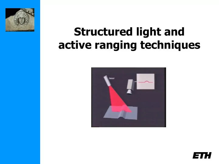
Structured light and active ranging techniques

3D photography course schedule

Topic

Feb 21 Introduction Feb 28 Lecture: Geometry, Camera Model, Calibration Mar 7 Lecture: Features & Correspondences Mar 14 Project Proposals Mar 21 Lecture: Epipolar Geometry Mar 28 Depth Estimation + 2 papers Apr 4 Single View Geometry + 2 papers Apr 11 Active Ranging and Structured Light + 2 papers Apr 18 Project Updates

• Apr. 25
• -- Easter ---

May 2 SLAM + 2 papers May 9 3D & Registration + 2 papers May 16 Structure from Motion + 2 papers May 23 Shape from Silhouettes + 2 papers May 30 Final Projects (if not demo day)

Today’s class

• unstructured light
• structured light
• time-of-flight

(some slides from Szymon Rusinkiewicz, Brian Curless)

A Taxonomy

A taxonomy

Unstructured light

project texture to disambiguate stereo

Space-time stereo

Davis, Ramamoothi, Rusinkiewicz, CVPR’03

Space-time stereo

Davis, Ramamoothi, Rusinkiewicz, CVPR’03

Space-time stereo

Zhang, Curless and Seitz, CVPR’03

Space-time stereo

• results

Zhang, Curless and Seitz, CVPR’03

Light Transport Constancy

Davis, Yang, Wang, ICCV05

Triangulation

Triangulation: Moving the Camera and Illumination

• Moving independently leads to problems

with focus, resolution

• Most scanners mount camera and light

source rigidly, move them as a unit, allows also for (partial) pre-calibration

Triangulation: Moving the Camera and Illumination

Triangulation: Moving the Camera and Illumination

(Rioux et al. 87)

Triangulation: Extending to 3D

• Possibility #1: add another mirror (flying spot)
• Possibility #2: project a stripe, not a dot

Object Laser Camera Camera

Triangulation Scanner Issues

• Accuracy proportional to working volume

(typical is ~1000:1)

• Scales down to small working volume

(e.g. 5 cm. working volume, 50 m. accuracy)

• Does not scale up (baseline too large…)
• Two-line-of-sight problem (shadowing from

either camera or laser)

• Triangulation angle: non-uniform resolution if

too small, shadowing if too big (useful range: 15-30)

Triangulation Scanner Issues

• Material properties (dark, specular)
• Subsurface scattering
• Laser speckle
• Edge curl
• Texture embossing

Space-time analysis

Curless ‘95

Space-time analysis

Curless ‘95

Projector as camera

Multi-Stripe Triangulation

• To go faster, project multiple stripes
• But which stripe is which?
• Answer #1: assume surface continuity

e.g. Eyetronics’ ShapeCam

Kinect

• Infrared „projector“
• Infrared camera
• Works indoors (no IR distraction)
• „invisible“ for human

Depth Map: note stereo shadows! Color Image (unused for depth) IR Image

Kinect

• Projector Pattern „strong texture“
• Correlation-based stereo

between IR image and projected pattern possible

stereo shadow Bad SNR / too close Homogeneous region, ambiguous without pattern

Multi-Stripe Triangulation

• To go faster, project multiple stripes
• But which stripe is which?
• Answer #2: colored stripes (or dots)

Multi-Stripe Triangulation

• To go faster, project multiple stripes
• But which stripe is which?
• Answer #3: time-coded stripes

Time-Coded Light Patterns

• Assign each stripe a unique illumination code
• ver time [Posdamer 82]

Space Time

Better codes…

• Gray code

Neighbors only differ one bit

Poor man’s scanner

Bouguet and Perona, ICCV’98

Pulsed Time of Flight

• Basic idea: send out pulse of light (usually laser),

time how long it takes to return t c d   2 1 t c d   2 1

Pulsed Time of Flight

• Advantages:
• Large working volume (up to 100 m.)
• Disadvantages:
• Not-so-great accuracy (at best ~5 mm.)
• Requires getting timing to ~30 picoseconds
• Does not scale with working volume
• Often used for scanning buildings, rooms,

archeological sites, etc.

Depth cameras

2D array of time-of-flight sensors

e.g. Canesta’s CMOS 3D sensor

jitter too big on single measurement, but averages out on many

(10,000 measurements100x improvement)

Depth cameras

Superfast shutter + standard CCD

• cut light off while pulse is

coming back, then I~Z

• but I~albedo (use

unshuttered reference view)

3DV’s Z-cam

AM Modulation Time of Flight

• Modulate light at frequencym , it returns with a

phase shift 

• Note the ambiguity in the measured phase!

 Range ambiguity of 1/2mn                     2 2 2 1 n ν c d

m

                    2 2 2 1 n ν c d

m

Mesa Swissranger

AM Modulation Time of Flight

• Accuracy / working volume tradeoff

(e.g., noise ~ 1/500 working volume)

• “wraparound”-effect 2π (very close/far objects!)
• In practice, often used for room-sized

environments (cheaper, more accurate than pulsed time of flight)

ToF Depth Cameras

• + fast/synchronized depth acquisition
• - limited range (~2-20m)
• - So far, very limited resolution (~200x200) and

very noisy

Shadow Moire

Next Monday: Project Updates !

Presentations

Scharstein/Szeliski: “High Accuracy Stereo Depth Maps using Structured Light” Valkenburg/McIvor: “Accurate 3D measurement using a Structured Light System”