
SLIDE 1
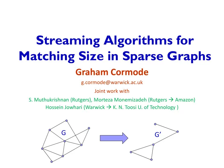
Streaming Algorithms for Matching Size in Sparse Graphs
Graham Cormode
g.cormode@warwick.ac.uk Joint work with
- S. Muthukrishnan (Rutgers), Morteza Monemizadeh (Rutgers Amazon)
Hossein Jowhari (Warwick K. N. Toosi U. of Technology )