
SLIDE 1
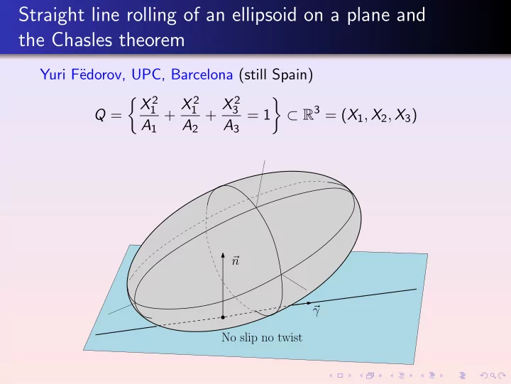
Straight line rolling of an ellipsoid on a plane and the Chasles theorem
Yuri F¨ edorov, UPC, Barcelona (still Spain) Q = X 2
1
A1 + X 2
1
A2 + X 2
3
A3 = 1
- ⊂ R3 = (X1, X2, X3)
- n
- γ
Straight line rolling of an ellipsoid on a plane and the Chasles - - PowerPoint PPT Presentation
Straight line rolling of an ellipsoid on a plane and the Chasles theorem Yuri F edorov, UPC, Barcelona (still Spain) X 2 + X 2 + X 2 R 3 = ( X 1 , X 2 , X 3 ) 1 1 3 Q = = 1 A 1 A 2 A 3 n No slip no twist The