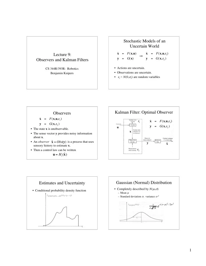
Stochastic Models of an Uncertain World x = F ( x , u ) x = F ( - PDF document

Stochastic Models of an Uncertain World ˙ ˙ x = F ( x , u ) x = F ( x , u , � 1 ) Lecture 9: � y G ( x ) y G ( x , � 2 ) = = Observers and Kalman Filters • Actions are uncertain. CS 344R/393R: Robotics • Observations are uncertain. Benjamin Kuipers • ε i ~ N (0, σ i ) are random variables Kalman Filter: Optimal Observer Observers ˙ x = F ( x , u , � 1 ) ˙ � x = F ( x , u , � 1 ) 1 y = G ( x , � 2 ) y = G ( x , � 2 ) u • The state x is unobservable. x • The sense vector y provides noisy information about x . • An observer is a process that uses x = Obs ( y ) ˆ y ˆ x sensory history to estimate x . � 2 • Then a control law can be written u = H i (ˆ x ) Gaussian (Normal) Distribution Estimates and Uncertainty • Completely described by N ( µ , σ ) • Conditional probability density function – Mean µ – Standard deviation σ , variance σ 2 � ( x � µ ) 2 / 2 � 2 1 2 � e � 1

A Second Observation Estimating a Value 2 • Suppose there is a constant value x . • At time t 2 , observe value z 2 with variance � 2 – Distance to wall; angle to wall; etc. 2 � 1 • At time t 1 , observe value z 1 with variance ˆ • The optimal estimate is with x ( t 1 ) = z 1 2 � 1 variance Merged Evidence Update Mean and Variance • Weighted average of estimates. ˆ x ( t 2 ) = Az 1 + Bz 2 A + B = 1 • The weights come from the variances. – Smaller variance = more certainty � � � � 2 2 � 2 � 1 ˆ � � � � x ( t 2 ) = z 1 + z 2 2 + � 2 2 + � 2 2 2 � � � � � 1 � 1 � � � � 2 ( t 2 ) = 1 1 2 + 1 2 � � 1 � 2 From Weighted Average Predictor-Corrector to Predictor-Corrector • Update best estimate given new data • Weighted average: ˆ ( t 2 ) = ˆ 1 ) + K ( t 2 )( z 2 � ˆ x x ( t x ( t 1 )) ˆ x ( t 2 ) = Az 1 + Bz 2 = (1 � K ) z 1 + Kz 2 2 � 1 K ( t 2 ) = 2 + � 2 2 � 1 • Predictor-corrector: • Update variance: ˆ x ( t 2 ) = z 1 + K ( z 2 � z 1 ) 2 ( t 2 ) = � 2 ( t 2 ( t � 1 ) � K ( t 2 ) � 1 ) = ˆ x ( t 1 ) + K ( z 2 � ˆ x ( t 1 )) 2 ( t = (1 � K ( t 2 )) � 1 ) – This version can be applied “recursively”. 2

Static to Dynamic Dynamic Prediction • Now suppose x changes according to 2 ( t 2 ) ˆ • At t 2 we know x ( t 2 ) � x = F ( x , u , � ) = u + � ˙ ( N (0, � � )) • At t 3 after the change, before an observation. � ) = ˆ ˆ x ( t 3 x ( t 2 ) + u [ t 3 � t 2 ] 2 ( t 3 2 ( t 2 ) + � � 2 [ t 3 � t 2 ] � ) = � � • Next, we correct this prediction with the observation at time t 3 . Qualitative Properties Dynamic Correction � ) + K ( t 3 )( z 3 � ˆ � )) ˆ ( t 3 ) = ˆ x x ( t 3 x ( t 3 2 • At time t 3 we observe z 3 with variance � 3 � 2 ( t 3 � ) K ( t 3 ) = • Combine prediction with observation. 2 ( t 3 2 � ) + � 3 � � ) + K ( t 3 )( z 3 � ˆ � )) ˆ ( t 3 ) = ˆ x x ( t 3 x ( t 3 2 • Suppose measurement noise is large. � 3 – Then K ( t 3 ) approaches 0, and the measurement 2 ( t 3 ) = ( 2 ( t 3 � ) 1 � K ( t 3 )) � � will be mostly ignored. 2 ( t 3 � ) • Suppose prediction noise is large. � � 2 ( t 3 � ) K ( t 3 ) = – Then K ( t 3 ) approaches 1, and the measurement 2 ( t 3 2 � ) + � 3 � will dominate the estimate. Simplifications Kalman Filter • We have only discussed a one-dimensional • Takes a stream of observations, and a system. dynamical model. – Most applications are higher dimensional. • At each step, a weighted average between • We have assumed the state variable is – prediction from the dynamical model observable. – correction from the observation. – In general, sense data give indirect evidence. • The Kalman gain K ( t ) is the weighting, ˙ x = F ( x , u , � 1 ) = u + � 1 2 ( t ) 2 – based on the variances and � � � z = G ( x , � 2 ) = x + � 2 2 ( t ) • With time, K ( t ) and tend to stabilize. � • We will discuss the more complex case next. 3