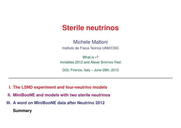
sterile neutrinos
play

Sterile neutrinos Michele Maltoni Instituto de F sica Te orica - PowerPoint PPT Presentation

Sterile neutrinos Michele Maltoni Instituto de F sica Te orica UAM/CSIC What is ? Invisibles 2012 and Alexei Smirnov Fest GGI, Firenze, Italy June 28th, 2012 I. The LSND experiment and four-neutrino models II. MiniBooNE and


  1. Sterile neutrinos Michele Maltoni Instituto de F´ ısica Te´ orica UAM/CSIC What is ν ? Invisibles 2012 and Alexei Smirnov Fest GGI, Firenze, Italy – June 28th, 2012 I. The LSND experiment and four-neutrino models II. MiniBooNE and models with two sterile neutrinos III. A word on MiniBooNE data after Neutrino 2012 Summary

  2. I. The LSND experiment and four-neutrino models 2 The LSND problem 10 2 • LSND observed ¯ ν e appearance in a ¯ ν µ beam ( E ν ∼ ∆ m 2 (eV 2 /c 4 ) 30 MeV, L ≃ 35 m); 10 • Karmen did not confirm the claim, but couldn’t fully Karmen CCFR exclude it either; Bugey 1 • the signal is compatible with ¯ ν µ → ¯ ν e oscillations NOMAD provided that ∆ m 2 � 0 . 1 eV 2 ; -1 10 • on the other hand, other data give (at 3 σ ): 90% (L max -L < 2.3) 99% (L max -L < 4.6)  ≃ 7 . 5 ± 0 . 6 × 10 − 5 eV 2 , ∆ m 2 -2 10 � ≃ 2 . 4 ± 0 . 3 × 10 − 3 eV 2 ; � � -3 -2 -1 � ∆ m 2 10 10 10 1 � � sin 2 2 θ  • in order to explain LSND with mass-induced neutrino oscillations one needs at least one more neutrino mass eigenstate; • WARNING: having enough ∆ m 2 is not enough. To make sure that the model works, one has to check explicitly that all the experiments can be fitted simultaneously. Michele Maltoni <michele.maltoni@csic.es> M  -  “W   ν ?”, 28/06/2012

  3. I. The LSND experiment and four-neutrino models 3 Four neutrino mass models • Approximation: ∆ m 2  ≪ ∆ m 2  ≪ ∆ m 2  ⇒ 6 different mass schemes: sol sol atm atm atm sol SBL SBL SBL SBL SBL SBL sol atm atm atm sol sol (a) (b) (c) (d) (A) (B)                   (3+1) (2+2) • Total: 3 ∆ m 2 , 6 angles, 3 phases. Different set of experimental data partially decouple : ∆ m 2 ∆ m 2 ∆ m 2 ϕ 13 SOL ATM LSND SOL η s ATM d µ NEV LSND ϕ 34 η e ϕ 12 θ SOL θ ATM θ LSND Michele Maltoni <michele.maltoni@csic.es> M  -  “W   ν ?”, 28/06/2012

  4. I. The LSND experiment and four-neutrino models 4 (2+2): ruled out by solar and atmospheric data 40 D D N N A A L L solar m solar (pre SNO salt) m global 2 χ 30 a a PG K K + + solar solar 2 χ Real 2 20 PC ∆χ atm Restricted + atm atm LBL 10 3 σ 3 σ 3 σ + + LBL + LBL SBL 0 0 0.2 0.4 0.6 0.8 1 0 0.2 0.4 0.6 0.8 1 0 0.2 0.4 0.6 0.8 1 η s η s = d s d s • in (2+2) models, fractions of ν s in solar ( η s ) and atmos ( 1 − d s ) add to one ⇒ η s = d s ; • 3 σ allowed regions η s ≤ 0 . 31 (solar) and d s ≥ 0 . 63 (atmos) do not overlap; superposition occurs only above 4 . 5 σ ( χ 2  = 19 . 9 ); • the χ 2 increase from the combination of solar and atmos data is χ 2  = 28 . 6 (1 dof), corresponding to a PG = 9 × 10 − 8 [1]. [1] M. Maltoni, T. Schwetz, M.A. Tortola, J.W.F . Valle, Nucl. Phys. B643 (2002) 321 [ hep-ph/0207157 ]. Michele Maltoni <michele.maltoni@csic.es> M  -  “W   ν ?”, 28/06/2012

  5. I. The LSND experiment and four-neutrino models 5 (3+1): tension between LSND and short-baseline data • In (3+1) schemes the SBL appearance probability is effectively 2 ν oscillations: 1 10 P µ e = sin 2 2 θ sin 2 ∆ m 2 41 L sin 2 2 θ = 4 | U e 4 | 2 | U µ 4 | 2 ; , ★ 2 ] 4 E 41 [eV LSND DAR (90%, 99%) • disappearance experiments bound | U e 4 | 2 and | U µ 4 | 2 ; 0 2 10 ∆ m 2 10 99% CL 9 0 % ★ -1 10 C atm + LBL + NEV L 1 10 CDHS -4 -3 -2 -1 0 10 10 10 10 10 2 ] 41 [eV 2 2 θ = 4 |U e4 | 2 |U µ 4 | 2 sin ★ Bugey 0 10 2 ∆ m • LSND is in conflict [1]: -1 10 atmospheric − with other appearance experi- Chooz ments (Karmen & Nomad); -2 10 -3 -2 -1 -3 -2 -1 10 10 10 10 10 10 2 2 − with all disappearance exp’s. |U e4 | |U µ 4 | [1] M. Maltoni, T. Schwetz, M.A. Tortola, J.W.F . Valle, Nucl. Phys. B643 (2002) 321 [ hep-ph/0207157 ]. Michele Maltoni <michele.maltoni@csic.es> M  -  “W   ν ?”, 28/06/2012

  6. I. The LSND experiment and four-neutrino models 6 The MiniBooNE experiment ( ≤ 5/2012) [MB- ¯ ν e ] • E ν and L very different from LSND (but similar L / E ν ) ⇒ can check the oscillation solution of the LSND problem, not the signal itself; • very peculiar results: − strong low-energy excess in ν e , mild in ¯ ν e ; − mild mid-energy excess in ¯ ν e , but not in ν e . 3 Data Events / MeV Predicted Spectrum ν Data 80 e from [MB- ν e ] ν µ 2.5 Uncertainty in Prediction e Events/(100 MeV) + ν from K ± Neutrinos from K ’s e 0 from K ν 0 Neutrinos from K ’s 60 2 e L 0 misid π Neutrinos from ’s µ ∆ → N γ Neutrinos from π ’s dirt 1.5 40 other Total Background 1 20 [NuMI- ν e ] 0.5 0 0.2 0.6 1 1.4 1.8 2.2 2.6 3 0.2 0.4 0.6 0.8 1 1.2 1.4 1.5 1.6 3. Reconstructed E [GeV] QE E (GeV) ν ν Michele Maltoni <michele.maltoni@csic.es> M  -  “W   ν ?”, 28/06/2012

  7. I. The LSND experiment and four-neutrino models 7 LSND vs MiniBooNE in (3+1) [ ¯ ν e ] • ν e : no signal ⇒ excludes LSND; ν e : signal ⇒ mildly confirms LSND. • ¯ 2 10 [ ν e ] 2 sin (2 θ ) upper limit MiniBooNE 90% C.L. y MiniBooNE 90% C.L. sensitivity 10 BDT analysis 90% C.L. ) 4 /c 2 | (eV 1 2 m ∆ | -1 10 LSND 90% C.L. LSND 99% C.L. -2 10 -3 -2 -1 10 10 10 1 2 sin (2 ) θ Michele Maltoni <michele.maltoni@csic.es> M  -  “W   ν ?”, 28/06/2012

  8. I. The LSND experiment and four-neutrino models 8 2 10 Status of (3+1) models after MiniBooNE (3+1) [2] 10 • (3+1) four-neutrino schemes fail because: ) 2 (eV 1 − can’t reconcile appearance and disappearance data; 41 2 m ∆ -1 10 − can’t explain the different ν e (MB) and ¯ ν e (LSND) results; null SBL 90% CL null SBL 99% CL − can’t account for the low-energy ν e event excess in MB. LSND + BNB-MB( ν ) + BNB-MB( ν ) 90% CL -2 10 LSND + BNB-MB( ) + BNB-MB( ) 99% CL ν ν -4 -3 -2 -1 10 10 10 10 1 ⇒ (3+1) models are ruled out as explanation of SBL data. 2 sin (2 ) θ µ e BNB-MB( ) BNB-MB( ) LSND ν ν [OLD] 2 2 2 10 10 10 [2] 90% CL 90% CL 90% CL 99% CL 99% CL 99% CL 10 10 10 ) ) ) 2 2 2 (eV (eV (eV 41 41 41 2 2 2 m 1 m 1 m 1 ∆ ∆ ∆ -1 -1 -1 10 10 10 -3 -2 -1 -3 -2 -1 -3 -2 -1 10 10 10 10 10 10 10 10 10 2 2 2 sin (2 ) sin (2 ) sin (2 ) θ θ θ µ e µ e µ e [2] G. Karagiorgi et al. , Phys. Rev. D80 (2009) 073001 [ arXiv:0906.1997 ]. Michele Maltoni <michele.maltoni@csic.es> M  -  “W   ν ?”, 28/06/2012

  9. II. MiniBooNE and models with two sterile neutrinos 9 3 The MiniBooNE excess Events / MeV Data ν from µ 2.5 e + from K ν e With the analysis cuts set, a signal-blind test of data- 0 from K ν 2 e MC agreement in the signal region was performed. The π 0 misid full two-neutrino oscillation fit was done in the range N ∆ → γ 300 < E QE < 3000 MeV and, with no information on dirt 1.5 ν the fit parameters revealed, the sum of predicted back- other ground and simulated best-fit signal was compared to Total Background 1 data in several variables, returning only the χ 2 . While agreement was good in most of the comparisons, the E vis spectrum had a χ 2 probability of only 1%. This triggered 0.5 further investigation of the backgrounds, focusing on the lowest energies where ν µ -induced backgrounds, some of which are difficult to model, are large. As part of this 0.2 0.4 0.6 0.8 1 1.2 1.4 1.5 1.6 3. study, one more piece of information from the signal re- QE E (GeV) gion was released: unsigned bin-by-bin fractional discrep- ν ancies in the E vis spectrum. While ambiguous, these re- inforced suspicions about the low-energy region. Though • MiniBooNE observed a 3 . 0 σ excess at low-E [3]; we found no specific problems with the background es- timates, it was found that raising the minimum E QE of ν • this excess is incompatible with 2 ν oscillations; the fit region to 475 MeV greatly reduced a number of backgrounds with little impact on the fit’s sensitivity to • therefore, data with E QE < 475 MeV have not oscillations. We thus performed our oscillation fits in the ν energy range 475 < E QE < 3000 MeV and opened the ν been used to check LSND. full data set. ⇒ Omission of low-energy bins in based on the hypothesis of two-flavor oscillations ! • Is it possible to do something about these data in more sophisticated models? [3] A.A. Aguilar-Arevalo et al. [MiniBooNE collab], Phys. Rev. Lett. 98 (2007) 231801 [arXiv:0704.1500]. Michele Maltoni <michele.maltoni@csic.es> M  -  “W   ν ?”, 28/06/2012

Download Presentation
Download Policy: The content available on the website is offered to you 'AS IS' for your personal information and use only. It cannot be commercialized, licensed, or distributed on other websites without prior consent from the author. To download a presentation, simply click this link. If you encounter any difficulties during the download process, it's possible that the publisher has removed the file from their server.

Recommend


More recommend