Statistics Intro One key difference between 262A and B is that this - PDF document

Advanced Topics in Computer Systems, CS262B Prof. Eric Brewer Statistics Intro One key difference between 262A and B is that this semester we will expect PhD level data analysis and presentation. This includes experimental design, data collection and measurement, and presentation with confidence intervals. In this lecture, we cover the basics, which will not be sufficient to deliver the above goals, but is a start. The difference will be made up as we go through the class projects. I. 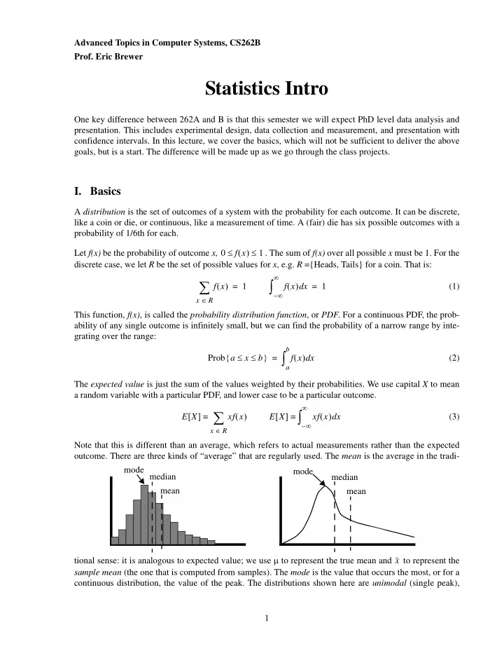Basics A distribution is the set of outcomes of a system with the probability for each outcome. It can be discrete, like a coin or die, or continuous, like a measurement of time. A (fair) die has six possible outcomes with a probability of 1/6th for each. ≤ ( ) ≤ Let f(x) be the probability of outcome x, 0 f x 1 . The sum of f(x) over all possible x must be 1. For the discrete case, we let R be the set of possible values for x , e.g. R ={Heads, Tails} for a coin. That is: ∞ ∑ ∫ ( ) ( ) x = 1 = 1 (1) f x f x d ∞ – ∈ x R This function, f(x) , is called the probability distribution function , or PDF . For a continuous PDF, the prob- ability of any single outcome is infinitely small, but we can find the probability of a narrow range by inte- grating over the range: b ∫ { ≤ ≤ } ( ) x Prob a x b = f x d (2) a The expected value is just the sum of the values weighted by their probabilities. We use capital X to mean a random variable with a particular PDF, and lower case to be a particular outcome. ∞ ∑ ∫ [ ] ≡ ( ) [ ] ≡ ( ) x E X xf x E X xf x d (3) ∞ – ∈ x R Note that this is different than an average, which refers to actual measurements rather than the expected outcome. There are three kinds of “average” that are regularly used. The mean is the average in the tradi- mode median mode median mean mean tional sense: it is analogous to expected value; we use μ to represent the true mean and to represent the x sample mean (the one that is computed from samples). The mode is the value that occurs the most, or for a continuous distribution, the value of the peak. The distributions shown here are unimodal (single peak), 1

bimodal distributions have two peaks. There is only one mode even for a bimodal distribution, although it is not clear what happens if there is a tie; in general, the mode is only used for unimodal distributions. The median is the value with half the values above it and half below it. In a continuous curve the (expected) median has half the area of the PDF is on each side. (A measured median is not a continuous curve, since it is just a collection of samples.) These two plots are skewed to the right, which means that they have a long tail to the right. With long tails, we expect mode < median < mean. A left-skewed distribution would have mean < median < mode. Any order is possible, since the mode can be on either side of the median, and since you can “stretch” the tail on one side or the other to move the mean without moving the mode or median. The variance measures the amount of variation in a distribution, in some sense, its “width”. It measures the average of the square of the distance from the mean for each value. Think of the “square” part as a way to remove the effect of whether the difference is positive or negative. ∞ ) 2 ∑ ) 2 f x ∫ ) 2 f x [ ] ≡ [ ( μ ] ( μ ( ) ( μ ( ) x – = – – (4) Variance X E X x x d ∞ – ∈ x R σ More useful and intuitive than the variance is the standard deviation , , which is just the square root of the σ 2 [ ] ≡ variance, so Variance x . Unlike variance, standard deviation has an intuitive definition: it is the average distance from the mean of the samples. Keep in mind that variance is based of the squares of the distances, and stddev is the square root of the variance, making it essentially the average of the distances. It is also useful to realize that the standard deviation is measured in the same units as the random variable; i.e. if the outcomes are measured in seconds, then so are the mean and standard deviation. This is why we can talk about confidence intervals (below) that are based on the mean and stddev. It is also useful to know that the expected value of a linear combination of variables is just the linear com- bination of the expected values, and there is a similar relationship for variance (but not stddev): … if Y = a 1 X 1 + a 2 X 2 + + a n X n then: (5) ∑ ∑ 2 Var X i [ ] [ ] [ ] [ ] E Y = a i E X i Var Y = a i i i II. Cumulative Distribution Functions Before we get to confidence intervals, we should define cumulative distribution functions , or CDFs . Every PDF has a corresponding CDF which is the cumulative sum of the probabilities up to the current point, which is the same as the probability that x is less than the current point. Using c(x) to mean the CDF corre- sponding to the PDF f(x) : a ∫ ( ) ≡ [ ≤ ] ≡ ( ) x c + ∞ ( ) ≡ ( ∞ ) ≡ ≤ ( ) ≤ c a Prob x a f x d 1 c – 0 0 c x 1 (6) ∞ – In practice, CDFs are only used for continuous PDFs, but they can be well defined for the discrete case if the values of the random variable are ordered. The main use of a CDF is that it can convert an integration over the PDF into a subtraction of two CDF values. For example, to find the probability that the outcome is between a and b : 2

b ∫ [ < ≤ ] ≡ ( ) x ( ) ( ) = – (7) Prob a x b f x d c b c a a < ≤ This is a really simple but important equation. Intuitively, think of it as “the probability that a x b ≤ ≤ equals the probability that x b minus the probability that x a .” In practice, we will look up the two CDF values in a table. Note also that: [ > ] ( ) Prob x a = 1 – c a (8) III. Normal Distribution The normal distribution is the most important one, in part because it is a key tool for confidence intervals. σ 2 We define N( μ,σ ) as the normal distribution with mean μ and variance : ( μ ) 2 x – - - - - - - - - - - - - - - - - - - - – 1 2 σ 2 N μ σ ( , ) ≡ - - - - - - - - - - - - - - e (9) 2 πσ This is a nasty looking integral, but fortunately the CDF table means we almost never have to deal with it. σ 2 If you are bored, you can prove that E[N] = μ , Var[N] = , and that the area under the curve is 1. We call N(0, 1) the standard normal distribution, and its CDF is Φ (x), which is the function we actually look up in a table. The graph below shows N and its CDF plotted against μ and σ : 1 0 .4 5 0 .4 0 .3 5 0 .3 0 .2 5 0 .2 0 .1 5 0 .1 0 .0 5 0 - 5 - 4 - 3 - 2 - 1 0 1 2 3 4 5 μ−2σ μ−σ μ μ+σ μ+2σ Since, Φ (x) is the CDF for N(0,1), we need a way to get the CDF for N( μ , σ ). Fortunately, this is just a lin- ear translation: μ μ ⎛ ⎞ ⎛ ⎞ Φ b – Φ a – [ < ≤ ] - - - - - - - - - - - - - - - - - - - - - - - - Prob a x b = – (10) ⎝ ⎠ ⎝ ⎠ σ σ 3

Thus, given a random variable with distribution N( μ , σ ), we have a way to compute the probability of any range using just two values from a standardized table. IV. Sampling So far we have only talked about distributions that are known a priori . In practice, we don’t really know the distribution, or at least not its parameters, and we have to deduce them from samples. The collection of samples is called the empirical distribution . The sample mean is average of the samples, typically represented as x , called “x-bar”. From (5), we deduce: ∑ 1 ≡ - - - x i x n (11) [ ] ⎛ ⎞ 2 n 1 1 Var X [ ] ⋅ [ ] μ [ ] ⋅ [ ] - - E X - - - - - - - - - - - - - - - - - - - - - - E x = = Var x = n Var X = ⎝ ⎠ n n n [ ] μ , we say that the sample mean is an unbiased estimator of μ . This assumes that the sam- Since E x = ples are independent and all taken from the same distribution, or iid for “independent and identically dis- tributed” (pronounced “eye-eye-dee”). This is a non-trivial assumption that is often wrong! For example, if you sample without replacement from a finite set, the distribution changes as you remove items. Steady- state systems typically have different distributions then the same system when it is warming up. Perhaps more interesting than the expected value is the variance. The variance of the sample mean decreases linearly as we add samples! This implies that the standard deviation of the sample mean decreases with the square root of the number of samples. This is why adding samples increases the accu- racy of the sample mean. This means, among other things, that if X is N( μ , σ ), then has the distribution x σ N( μ , - - - - - - - ). n At this point, it is worth mentioning that you can compute the sample mean and variance as you go, rather than waiting until you have all of the samples. There is an alternate (equivalent) definition of variance that is more useful for this purpose, as it is easy to use as part of a running sum: ⎛ ⎞ 2 1 ∑ 1 ∑ E X 2 μ 2 E X 2 ) 2 2 [ ] [ ] [ ] ( [ ] ⎜ ⎟ - - - - Variance X = – = – E X = x i – x i (12) n ⎝ n ⎠ i i x 2 Using this definition, if we keep a running sum of n , and then we can at any point calculate the sam- x ple mean and the variance for the samples so far. This is great for online systems, or systems looking for only good approximations, since they can wait until the variance drops below some threshold. 4