[PDF] - Statistical revolution in computational linguistics Speech PDF Document

SLIDE 1

Statistics and the Scientific Study of Language

What do they have to do with each other? Mark Johnson

Brown University

ESSLLI 2005

Outline

Why Statistics? Learning probabilistic context-free grammars Factoring learning into simpler components The Janus-faced nature of computational linguistics Conclusion

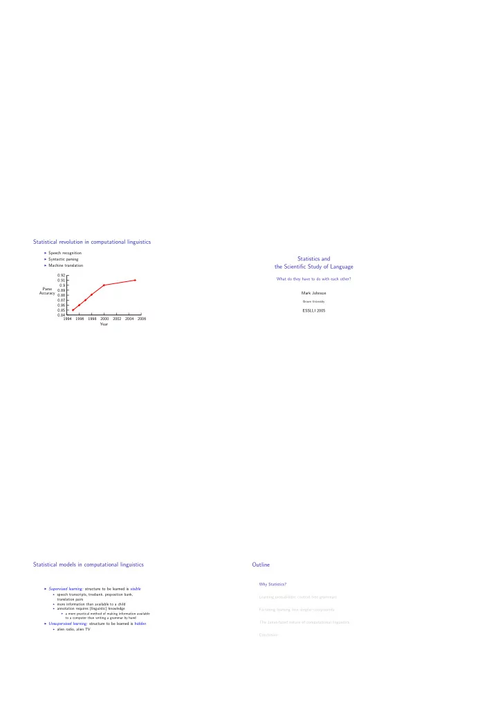
Statistical revolution in computational linguistics

◮ Speech recognition ◮ Syntactic parsing ◮ Machine translation

Year Parse Accuracy 2006 2004 2002 2000 1998 1996 1994 0.92 0.91 0.9 0.89 0.88 0.87 0.86 0.85 0.84

Statistical models in computational linguistics

◮ Supervised learning: structure to be learned is visible ◮ speech transcripts, treebank, proposition bank,

translation pairs

◮ more information than available to a child ◮ annotation requires (linguistic) knowledge ◮ a more practical method of making information available

to a computer than writing a grammar by hand

◮ Unsupervised learning: structure to be learned is hidden ◮ alien radio, alien TV

SLIDE 2

Chomsky’s “Three Questions”

◮ What constitutes knowledge of language? ◮ grammar (universal, language specific) ◮ How is knowledge of language acquired? ◮ language acquisition ◮ How is knowledge of language put to use? ◮ psycholinguistics

(last two questions are about inference)

The centrality of inference

◮ “poverty of the stimulus”

⇒ innate knowledge of language (universal grammar) ⇒ intricate grammar with rich deductive structure

The centrality of inference

◮ “poverty of the stimulus”

⇒ innate knowledge of language (universal grammar) ⇒ intricate grammar with rich deductive structure

◮ Statistics is the theory of optimal inference in the

presence of uncertainty

◮ We can define probability distributions over structured

bjects

⇒ no inherent contradiction between statistical inference and linguistic structure

◮ probabilistic models are declarative ◮ probabilistic models can be systematically combined

P(X, Y ) = P(X)P(Y |X)

Questions that statistical models might answer

◮ What information is required to learn language? ◮ How useful are different kinds of information to language

learners?

◮ Bayesian inference can utilize prior knowledge ◮ Prior can encode “soft” markedness preferences and

“hard” universal constraints

◮ Are there synergies between different information

sources?

◮ Does knowledge of phonology or morphology make word

segmentation easier?

◮ May provide hints about human language acquisition

SLIDE 3

Outline

Why Statistics? Learning probabilistic context-free grammars Factoring learning into simpler components The Janus-faced nature of computational linguistics Conclusion

Probabilistic Context-Free Grammars

1.0 S → NP VP 1.0 VP → V 0.75 NP → George 0.25 NP → Al 0.6 V → barks 0.4 V → snores P     

S NP VP George V barks

     = 0.45 P     

S NP VP Al V snores

     = 0.1

Estimating PCFGs from visible data

S NP VP rice grows S NP VP rice grows S NP VP corn grows

Rule Count Rel Freq S → NP VP 3 1 NP → rice 2 2/3 NP → corn 1 1/3 VP → grows 3 1 Rel freq is maximum likelihood estimator (selects rule probabilities that maximize probability of trees) P    

S NP VP rice grows

    = 2/3 P    

S NP VP corn grows

    = 1/3

Estimating PCFGs from hidden data

◮ Training data consists of strings w alone ◮ Maximum likelihood selects rule probabilities that

maximize the marginal probability of the strings w

◮ Expectation maximization is a way of building hidden

data estimators out of visible data estimators

◮ parse trees of iteration i are training data for rule

probabilities at iteration i + 1

◮ Each iteration is guaranteed not to decrease P(w) (but

can get trapped in local minima)

◮ This can be done without enumerating the parses

SLIDE 4

Example: The EM algorithm with a toy PCFG

Initial rule probs

rule prob · · · · · · VP → V 0.2 VP → V NP 0.2 VP → NP V 0.2 VP → V NP NP 0.2 VP → NP NP V 0.2 · · · · · · Det → the 0.1 N → the 0.1 V → the 0.1 “English” input the dog bites the dog bites a man a man gives the dog a bone · · · “pseudo-Japanese” input the dog bites the dog a man bites a man the dog a bone gives · · ·

Probability of “English”

Iteration Geometric average sentence probability 5 4 3 2 1 1 0.1 0.01 0.001 1e-04 1e-05 1e-06

Rule probabilities from “English”

V →the N →the Det →the VP →NP NP V VP →V NP NP VP →NP V VP →V NP Iteration Rule probability 5 4 3 2 1 1 0.9 0.8 0.7 0.6 0.5 0.4 0.3 0.2 0.1

Probability of “Japanese”

Iteration Geometric average sentence probability 5 4 3 2 1 1 0.1 0.01 0.001 1e-04 1e-05 1e-06

SLIDE 5

Rule probabilities from “Japanese”

V →the N →the Det →the VP →NP NP V VP →V NP NP VP →NP V VP →V NP Iteration Rule probability 5 4 3 2 1 1 0.9 0.8 0.7 0.6 0.5 0.4 0.3 0.2 0.1

Learning in statistical paradigm

◮ The likelihood is a differentiable function of rule

probabilities ⇒ learning can involve small, incremental updates

◮ Learning structure (rules) is hard, but . . . ◮ Parameter estimation can approximate rule learning ◮ start with “superset” grammar ◮ estimate rule probabilities ◮ discard low probability rules ◮ Parameters can be associated with other things besides

rules (e.g., HeadInitial, HeadFinal)

Applying EM to real data

◮ ATIS treebank consists of 1,300 hand-constructed parse

trees

◮ ignore the words (in this experiment) ◮ about 1,000 PCFG rules are needed to build these trees S VP VB Show NP PRP me NP NP PDT all DT the JJ nonstop NNS flights PP PP IN from NP NNP Dallas PP TO to NP NNP Denver ADJP JJ early PP IN in NP DT the NN morning . .

Experiments with EM

1. Extract productions from trees and estimate probabilities

probabilities from trees to produce PCFG.

2. Initialize EM with the treebank grammar and MLE

probabilities

3. Apply EM (to strings alone) to re-estimate production

probabilities.

4. At each iteration:

◮ Measure the likelihood of the training data and the

quality of the parses produced by each grammar.

◮ Test on training data (so poor performance is not due to

verlearning).

SLIDE 6

Log likelihood of training strings

Iteration log P 20 15 10 5

14000
14200
14400
14600
14800
15000
15200
15400
15600
15800
16000

Quality of ML parses

Recall Precision Iteration Parse Accuracy 20 15 10 5 1 0.95 0.9 0.85 0.8 0.75 0.7

Why does it work so poorly?

◮ Wrong data: grammar is a transduction between form

and meaning ⇒ learn from form/meaning pairs

◮ exactly what contextual information is available to a

language learner?

◮ Wrong model: PCFGs are poor models of syntax ◮ Wrong objective function: Maximum likelihood makes the

sentences as likely as possible, but syntax isn’t intended to predict sentences (Klein and Manning)

◮ How can information about the marginal distribution of

strings P(w) provide information about the conditional distribution of parses t given strings P(t|w)?

◮ need additional linking assumptions about the

relationship between parses and strings

◮ . . . but no one really knows!

Outline

Why Statistics? Learning probabilistic context-free grammars Factoring learning into simpler components The Janus-faced nature of computational linguistics Conclusion

SLIDE 7

Factoring the language learning problem

◮ Factor the language learning problem into linguistically

simpler components

◮ Focus on components that might be less dependent on

context and semantics (e.g., word segmentation, phonology)

◮ Identify relevant information sources (including prior

knowledge, e.g., UG) by comparing models

◮ Combine components to produce more ambitious learners ◮ PCFG-like grammars are a natural way to formulate many

f these components

Joint work with Sharon Goldwater and Tom Griffiths

Word Segmentation

Data = t h e d o g b a r k s

Utterance Word t h e Utterance Word d

g

Utterance Word b a r k s

Utterance → Word Utterance Utterance → Word Word → w w ∈ Σ⋆

◮ Algorithms for word segmentation from this information

already exists (e.g., Elman, Brent)

◮ Likely that children perform some word segmentation

before they know the meanings of words

Concatenative morphology

Data = t a l k i n g

Verb Stem t a l k Suffix i n g

Verb → Stem Suffix Stem → w w ∈ Σ⋆ Suffix → w w ∈ Σ⋆

◮ Morphological alternation provides primary evidence for

phonological generalizations (“trucks” /s/ vs. “cars” /z/)

◮ Morphemes may also provide clues for word segmentation ◮ Algorithms for doing this already exist (e.g., Goldsmith)

PCFG components can be integrated

Utterance WordsN N StemN d

g

SuffixN s WordsV V StemV b a r k SuffixV

Utterance → WordsS S ∈ S WordsS → S WordsT T ∈ S S → StemS SuffixS StemS → t t ∈ Σ⋆ SuffixS → f f ∈ Σ⋆

SLIDE 8

Problems with maximum likelihood estimation

◮ Maximum likelihood picks model that best fits the data ◮ Saturated models exactly mimic the training data

⇒ highest likelihood

◮ Need a different estimation framework

Utterance Word t h e d

g

b a r k s Verb Stem t a l k i n g Suffix

Bayesian estimation

P(Hypothesis|Data)

Posterior

∝ P(Data|Hypothesis)

Likelihood

P(Hypothesis)

Prior

◮ Priors can be sensitive to linguistic structure (e.g., a word

should contain a vowel)

◮ Priors can encode linguistic universals and markedness

preferences (e.g., complex clusters appear at word onsets)

◮ Priors can prefer sparse solutions ◮ The choice of the prior is as much a linguistic issue as the

design of the grammar!

Morphological segmentation experiment

◮ Trained on orthographic verbs from U Penn. Wall Street

Journal treebank

◮ Dirichlet prior prefers sparse solutions (sparser solutions

as α → 0)

◮ Gibbs Sampler used to sample from posterior distribution

f parses

◮ reanalyses each word based on a grammar estimated

from the parses of the other words

Posterior samples from WSJ verb tokens

α = 0.1 α = 10−5 α = 10−10 α = 10−15 expect expect expect expect expects expects expects expects expected expected expected expected expecting expect ing expect ing expect ing include include include include includes includes includ es includ es included included includ ed includ ed including including including including add add add add adds adds adds add s added added add ed added adding adding add ing add ing continue continue continue continue continues continues continue s continue s continued continued continu ed continu ed continuing continuing continu ing continu ing report report report report

SLIDE 9

Log posterior of models on token data

Posterior True suffixes Null suffixes Dirichlet prior parameter α log Pα 1 1e-10 1e-20

800000
1e+06
1.2e+06

◮ Correct solution is nowhere near as likely as posterior

⇒ model is wrong!

Independence assumption in PCFG model

Verb Stem t a l k Suffix i n g

P(Word) = P(Stem)P(Suffix)

◮ Model expects relative frequency of each suffix to be the

same for all stems

Relative frequencies of inflected verb forms Types and tokens

◮ A word type is a distinct word shape ◮ A word token is an occurrence of a word

Data = “the cat chased the other cat” Tokens = “the” 2, “cat” 2, “chased” 1, “other” 1 Types = “the” 1, “cat” 1, “chased” 1, “other” 1

◮ Using word types instead of word tokens effectively

normalizes for frequency variations

SLIDE 10

Posterior samples from WSJ verb types

α = 0.1 α = 10−5 α = 10−10 α = 10−15 expect expect expect exp ect expects expect s expect s exp ects expected expect ed expect ed exp ected expect ing expect ing expect ing exp ecting include includ e includ e includ e include s includ es includ es includ es included includ ed includ ed includ ed including includ ing includ ing includ ing add add add add adds add s add s add s add ed add ed add ed add ed adding add ing add ing add ing continue continu e continu e continu e continue s continu es continu es continu es continu ed continu ed continu ed continu ed continuing continu ing continu ing continu ing report report repo rt rep

rt

Summary so far

◮ Unsupervised learning is difficult on real data! ◮ There’s a lot to learn from simple problems ◮ need models that require all stems in same class to have

same suffixes but permit suffix frequencies to vary with the stem

◮ Related problems arise in other linguistic domains as well ◮ Many verbs share the same subcategorization frames,

but subcategorization frame frequencies depend on head verb.

◮ Hopefully we can combine these simple learners to study

their interaction in more complex domains

Outline

Why Statistics? Learning probabilistic context-free grammars Factoring learning into simpler components The Janus-faced nature of computational linguistics Conclusion

Psalter Mappa Mundi (1225?)

SLIDE 11

Portolan chart circa 1424 Portolan chart circa 1424 (center) Waldseem¨ uller 1507, after Ptolemy Battista Agnese portolan chart circa 1550

SLIDE 12

Mercator 1569 ... back to computational linguistics

◮ Be wary of analogies from the history of science! ◮ we only remember the successes ◮ May wind up learning something very different to what

you hoped

◮ Cartography and geography benefited from both the

academic and Portolan traditions

◮ Geography turned out to be about brute empirical facts ◮ but geology and plate tectonics ◮ Mathematics (geometry and trigonometry) turned out to

be essential

◮ Even wrong ideas can be very important ◮ the cosmographic tradition survives in celestial

navigation

Outline

Why Statistics? Learning probabilistic context-free grammars Factoring learning into simpler components The Janus-faced nature of computational linguistics Conclusion

Conclusion

◮ Statistical methods have both engineering and scientific

applications

◮ Inference plays a central role in linguistic theory ◮ Uncertain information ⇒ statistical inference ◮ The statistical component of a model may require as

much linguistic insight as the structural component

◮ Factoring the learning problem into linguistically simpler

pieces may be a good way to proceed

◮ Who knows what the future will bring?

SLIDE 13

Thank you

“I ask you to look both ways. For the road to a knowledge of the stars leads through the atom; and important knowledge of the atom has been reached through the stars.” — Sir Arthur Eddington “Everything should be made as simple as possible, but not one bit simpler.” — Albert Einstein “Something unknown is doing we don’t know what.” — Sir Arthur Eddington “You can observe a lot just by watching.” — Yogi Berra

Log posterior of models on type data

Optimal suffixes True suffixes Null suffixes Dirichlet prior parameter α log Pα 1 1e-10 1e-20

200000
400000

◮ Correct solution is close to optimal for α = 10−3

Morpheme frequencies provide useful information

Yarowsky and Wicentowski (2000) “Minimally supervised Morphological Analysis by Multimodal Alignment”

Suffix frequency depends on stem

Word V t a l k SuffixVtalk i n g

Word → S S ∈ S S → t SuffixS,t t ∈ Σ⋆ SuffixS,t → f f ∈ Σ⋆

◮ Suffix distributions SuffixS,t → f depend on the stem t ◮ Prior constrains suffix distributions SuffixS,t → f for

stems t in the same class to be similar

◮ Model is saturated and not context-free

SLIDE 14

Dirichlet priors and sparse solutions

◮ The expansions of a nonterminal in a PCFG are

distributed according to a multinomial

◮ Dirichlet priors are a standard prior over multinomial

distributions P(p1, . . . , pn) ∝

n

i=1

pα−1

i

α > 0

α = 2.0 α = 1.0 α = 0.5 α = 0.1 Binomial probability p Pα(p) 1 0.8 0.6 0.4 0.2 3 2 1

Estimation procedures

◮ Dirichlet prior prefers sparse solutions ⇒ MAP grammar

may be undefined even though MAP parses are defined

◮ Markov Chain Monte Carlo techniques can sample from

the posterior distribution over grammars and parses

◮ Gibbs sampling:

1. Construct a corpus of (word,tree) pairs by randomly

assigning trees to each word in the data

2. Repeat:

2.1 Pick a word w and its tree from the corpus at random 2.2 Estimate a grammar from the trees assigned to the

ther words in the corpus

2.3 Parse w with this grammar, producing a distribution

ver trees

2.4 Select a tree t from this distribution, and add (w, t) to the corpus

Outline

Why Statistics? Learning probabilistic context-free grammars Factoring learning into simpler components The Janus-faced nature of computational linguistics Conclusion

Maximum likelihood estimation from visible data

Correct parses for training data sentences All possible parses for all possible sentences

◮ Standard maximum likelihood estimation makes the

treebank trees t and strings w as likely as possible relative to all other possible trees and strings

g = arg max

g

= Pg(w, t) = arg max

g

Pg(t|w) Pg(w)

SLIDE 15

Maximum likelihood estimation from hidden data

for training data sentences All possible parses for training data sentences Correct parses All possible parses for all possible sentences

◮ Maximum likelihood estimation maximizes the probability

f the words w of the training data, relative to all other

possible word strings

g = arg max

g

Pg(w) = arg max

g

t

Pg(t, w)

Conditional MLE from visible data

Correct parses for training data sentences All possible parses for training data sentences All possible parses for all possible sentences

◮ Conditional MLE maximizes the conditional probability

Pg(t|w) of the training trees t relative to the training words w

◮ learns nothing from the distribution Pg(w) of words

Language as a transduction from form to meaning

Language

Representations Phonological Semantic Cognition A.I. representations S W

◮ Grammar generates a phonological form w from a

semantic representation s P(w, s) = Pg(w|s)

“language′′

Pc(s)

“cognition′′

Interpretation is finding the most likely meaning s⋆

w S W s⋆(w)

s⋆(w) = arg max

s∈S P(s|w) = arg max s∈S Pg(w|s)Pc(s)

SLIDE 16

Maximum likelihood estimate g from visible data

w s S W

◮ Training data consists of phonology/semantic pairs (w, s) ◮ Maximum likelihood estimate of grammar

g makes (w, s) as likely as possible relative to all other possible pairs (w ′, s′), w ′ ∈ W, s′ ∈ S

g = arg max

g

P(w, s) = arg max

g

P(w|s)

MLE g from hidden data

w s S W

◮ Training data consists of phonological strings w alone ◮ MLE makes w as likely as possible relative to other strings

g = arg max

g

P(w) = arg max

g

s∈S

Pg(w|s)Pc(s) ⇒ It may be possible to learn g from strings alone

◮ The cognitive model Pc can in principle be learnt the

same way