[PDF] - Statistical Natural Language Processing Recap: perceptron algorithm PDF Document

SLIDE 1

Statistical Natural Language Processing

Artifjcial Neural networks & deep learning Çağrı Çöltekin

University of Tübingen Seminar für Sprachwissenschaft

Summer Semester 2018

Preliminaries ANNs Deep ANNs CNNs RNNs Autoencoders

Artifjcial neural networks

Artifjcial neural networks (ANNs) are machine learning

models inspired by biological neural networks

ANNs are powerful non-linear models
Power comes with a price: there are no guarantees of

fjnding a global minimum of the error function

ANNs have been used in ML, AI, Cognitive science since

1950’s – with some ups and downs

Currently they are the driving force behind the popular

‘deep learning’ methods

Ç. Çöltekin, SfS / University of Tübingen Summer Semester 2018 1 / 72 Preliminaries ANNs Deep ANNs CNNs RNNs Autoencoders

The biological neuron

(showing a picture of a real neuron is mandatory in every ANN lecture)

Dendrite Soma Axon Axon terminall

Ç. Çöltekin, SfS / University of Tübingen Summer Semester 2018 2 / 72 Preliminaries ANNs Deep ANNs CNNs RNNs Autoencoders

Artifjcial and biological neural networks

ANNs are inspired by biological neural networks
Similar to biological networks, ANNs are made of many

simple processing units

Despite the similarities, there are many difgerences: ANNs

do not mimic biological networks

ANNs are a practical statistical machine learning methods

Ç. Çöltekin, SfS / University of Tübingen Summer Semester 2018 3 / 72 Preliminaries ANNs Deep ANNs CNNs RNNs Autoencoders

Recap: the perceptron

y = f  

m

∑

j

wjxj   where f(x) = { +1 if wx > 0 −1

therwise

In ANN-speak f(·) is called an activation function. x2 x1 . . . xm w

1

w2 wm y x0 = 1 w0

Ç. Çöltekin, SfS / University of Tübingen Summer Semester 2018 4 / 72 Preliminaries ANNs Deep ANNs CNNs RNNs Autoencoders

Recap: perceptron algorithm

w

Perceptron algorithm

minimizes the function J(w) = ∑

i

max(0, −wxiyi)

The online version picks

an misclassifjed example, and sets w ← w + xiyi

Algorithm is guaranteed to

converge if classes are linearly separable

Ç. Çöltekin, SfS / University of Tübingen Summer Semester 2018 5 / 72 Preliminaries ANNs Deep ANNs CNNs RNNs Autoencoders

Recap: logistic regression

P(y) = f  

m

∑

j

wjxj   where f(x) = 1 1 + e−wx x2 x1 . . . xm w

1

w2 wm P(y) x0 = 1 w0

Ç. Çöltekin, SfS / University of Tübingen Summer Semester 2018 6 / 72 Preliminaries ANNs Deep ANNs CNNs RNNs Autoencoders

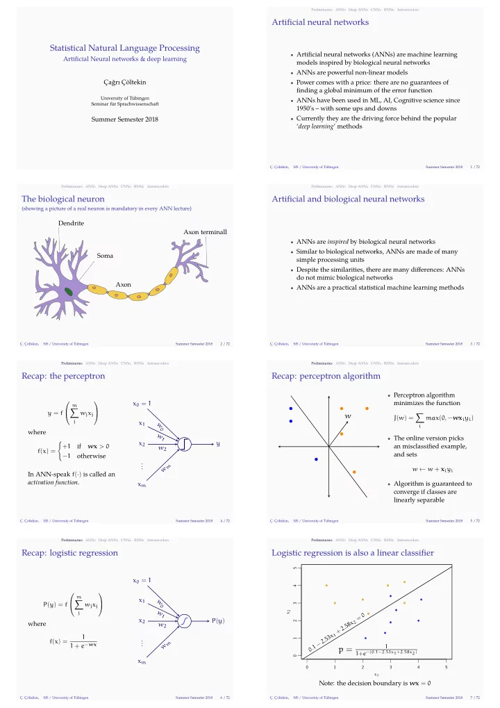
Logistic regression is also a linear classifjer

1 2 3 4 5 1 2 3 4 5 x1 x2

. 1 − 2 . 5 3 x

1

+ 2 . 5 8 x

2

=

p =

1 1+e−(0.1−2.53x1+2.58x2)

Note: the decision boundary is wx = 0

Ç. Çöltekin, SfS / University of Tübingen Summer Semester 2018 7 / 72

SLIDE 2

Preliminaries ANNs Deep ANNs CNNs RNNs Autoencoders

Linear separability

A classifjcation problem is

said to be linearly separable if one can fjnd a linear discriminator

A well-known counter

example is the logical XOR problem x2 x1 1 1 − + + − There is no line that can separate positive and negative classes.

Ç. Çöltekin, SfS / University of Tübingen Summer Semester 2018 8 / 72 Preliminaries ANNs Deep ANNs CNNs RNNs Autoencoders

Can a linear classifjer learn the XOR problem?

We can use non-linear basis functions

w0 + w1x1 + w2x2 + w3φ(x1, x2) is still linear in w for any choice of φ(·)

For example, adding the product x1x2 as an additional

feature would allow a solution like: x1 + x2 − 2x1x2 x1 x2 x1 + x2 − 2x1x2 1 1 1 1 1 1

Choosing proper basis functions like x1x2 is called feature

engineering

Ç. Çöltekin, SfS / University of Tübingen Summer Semester 2018 9 / 72 Preliminaries ANNs Deep ANNs CNNs RNNs Autoencoders

Multi-layer perceptron

The simplest modern ANN architecture is called

multi-layer perceptron (MLP)

(MLP) is a fully connected, feed-forward network consisting of

perceptron-like units

Unlike perceptron, the units in an MLP use a continuous

activation function

The MLP can be trained using gradient-based methods
The MLP can represent many interesting machine learning

problems

– It can be used for both regression and classifjcation

Ç. Çöltekin, SfS / University of Tübingen Summer Semester 2018 10 / 72 Preliminaries ANNs Deep ANNs CNNs RNNs Autoencoders

Multi-layer perceptron

the picture

x1 x2 x3 x4 y Input Hidden Output Each unit takes a weighted sum of their input, and applies a (non-linear) activation function.

Ç. Çöltekin, SfS / University of Tübingen Summer Semester 2018 11 / 72 Preliminaries ANNs Deep ANNs CNNs RNNs Autoencoders

An artifjcial neuron

∑ f(·) x2 x1 . . . xm w1 w2 wm y x0 = 1 w0

The unit calculates a

weighted sum of the inputs

m

∑

j

wjxj = wx

Result is a linear

transformation

Then the unit applies a

non-linear activation function f(·)

Output of the unit is

y = f(wx)

Ç. Çöltekin, SfS / University of Tübingen Summer Semester 2018 12 / 72 Preliminaries ANNs Deep ANNs CNNs RNNs Autoencoders

Artifjcial neuron

an example

∑ x2 x1 . . . xm w

1

w2 wm y x0 = 1 w0

A common activation

function is logistic sigmoid function f(x) = 1 1 + e−x

The output of the network

becomes y = 1 1 + e−wx

Ç. Çöltekin, SfS / University of Tübingen Summer Semester 2018 13 / 72 Preliminaries ANNs Deep ANNs CNNs RNNs Autoencoders

Activation functions in ANNs

hidden units

The activation functions in MLP are typically continuous

(difgerentiable) functions

For hidden units common choices are

Sigmoid (logistic)

1 1+ex

Hyperbolic tangent (tanh)

e2x−1 e2x+1

Rectifjed linear unit (relu) max(0, x)

Ç. Çöltekin, SfS / University of Tübingen Summer Semester 2018 14 / 72 Preliminaries ANNs Deep ANNs CNNs RNNs Autoencoders

Activation functions in ANNs

utput units
The activation functions of the output units depends on

the task

– For regression, identity function – For binary classifjcation, logistic sigmoid P(y = 1 | x) = 1 1 + e−wx = ewx 1 + e−wx – For multi-class classifjcation, softmax P(y = k | x) = ewkx ∑

j ewjx

Ç. Çöltekin, SfS / University of Tübingen Summer Semester 2018 15 / 72

SLIDE 3

Preliminaries ANNs Deep ANNs CNNs RNNs Autoencoders

MLP: a simple example

x1 x2 h1 h2 y1 y2 f() g() w(1)

11

w(1)

12

w(1)

21

w(1)

22

w(2)

11

w

( 2 ) 2 1

w

( 2 ) 1 2

w(2)

22

hj = f (∑

i

wijxi ) yk = g  ∑

j

wjkhj   yk = g  ∑

j

wjkf (∑

i

wijxi ) 

Ç. Çöltekin, SfS / University of Tübingen Summer Semester 2018 16 / 72 Preliminaries ANNs Deep ANNs CNNs RNNs Autoencoders

MLP: a simple example

x1 x2 h1 h2 y1 y2 f() g() w(1)

11

w(1)

12

w(1)

21

w(1)

22

w(2)

11

w

( 2 ) 2 1

w

( 2 ) 1 2

w(2)

22

Alternatively, we can write

the computations in matrix form h = f(W(1)x) y = g(W(2)h) = g ( W(2)f(W(1)x) )

This corresponds to a

series of transformations followed by element-wise (non-linear) function applications

Ç. Çöltekin, SfS / University of Tübingen Summer Semester 2018 17 / 72 Preliminaries ANNs Deep ANNs CNNs RNNs Autoencoders

Solving non-linear problems with ANNs

a solution to XOR problem

x1 h1 y x2 h2

f(z) = z2 g(z) =

1 1+e−z

1 1

h1 = ax1 + cx2 h2 = bx1 + dx2 y = eh1 + fh2 = (ea + fb)x1 + (ec + fd)x2 y is still a linear function of xi

Ç. Çöltekin, SfS / University of Tübingen Summer Semester 2018 19 / 72

SLIDE 4

Preliminaries ANNs Deep ANNs CNNs RNNs Autoencoders

Where do non-linearities come from?

non-linearities are abundant in nature, it is not only the XOR problem

In a linear model, y = w0 + w1x1 + . . . + wkxk

The outcome is linearly-related to the predictors
The efgects of the inputs are additive

This is not always the case:

Some predictors afgect the outcome in a non-linear way

– The efgect may be strong or positive only in a certain range

f the variable (e.g., reaction time change by age)

– Some efgects are periodic (e.g., many measures of time)

Some predictors interact

‘not bad’ is not ‘not’ + ‘bad’ (e.g., for sentiment analysis)

Ç. Çöltekin, SfS / University of Tübingen Summer Semester 2018 20 / 72 Preliminaries ANNs Deep ANNs CNNs RNNs Autoencoders

Finding the minimum of a loss function

Derivative of a function points to

the largest direction of change

Derivative is 0 at

minima/maxima

To fjnd the minimum (or

maximum) of error function f(x), we solve f′(x) = 0, for x

If no analytic solution exist, we

search for the minimum iteratively

−f′(x) for any x points towards

the minimum

Ç. Çöltekin, SfS / University of Tübingen Summer Semester 2018 21 / 72 Preliminaries ANNs Deep ANNs CNNs RNNs Autoencoders

Gradient descent: a refresher

The general idea is to approach a minimum of the error

function in small steps w ← w − η∇J(w)

– ∇J is the gradient of the loss function, it points to the direction of the maximum increase – η is the learning rate

The updates can be performed

batch for the complete training set

n-line after every training instance

– this is known as stochastic gradient descent (SGD) mini-batch after small fjxed-sized batches

Ç. Çöltekin, SfS / University of Tübingen Summer Semester 2018 22 / 72 Preliminaries ANNs Deep ANNs CNNs RNNs Autoencoders

Gradient descent: the picture

X ∇f(x1, . . . , xn) = ( ∂f ∂x1 , . . . , ∂f ∂xn )

Ç. Çöltekin, SfS / University of Tübingen Summer Semester 2018 23 / 72 Preliminaries ANNs Deep ANNs CNNs RNNs Autoencoders

Global and local minima

w E(w) local minimum global minimum

A function is convex if there is only one (global) minimum.

Ç. Çöltekin, SfS / University of Tübingen Summer Semester 2018 24 / 72 Preliminaries ANNs Deep ANNs CNNs RNNs Autoencoders

Error functions in ANN training

depend on the task

If we assume Gaussian noise, a natural choice is the

minimizing the sum of squared error E(w) = ∑

i

(yi − ˆ yi)2

For binary classifjcation, we use cross entropy

E(w) = − ∑

i

yi log ˆ yi + (1 − yi) log(1 − ˆ yi)

Similarly, for multi-class classifjcation, also cross entropy

E(w) = − ∑

i

∑

k

yi,k log ˆ yk In practice, the ANN loss functions will not be convex.

Ç. Çöltekin, SfS / University of Tübingen Summer Semester 2018 25 / 72 Preliminaries ANNs Deep ANNs CNNs RNNs Autoencoders

Learning in ANNs

ANNs implement complex functions: we need to use
ptimization methods (e.g., gradient descent) to train them
Typically error functions for ANNs are not convex,

gradient descent will fjnd a local minimum

Optimization requires updating multiple layers of weights
Assigning credit (or blame) to each weight during learning

is not trivial

An efgective solution to the last problem is the

backpropagation algorithm

Ç. Çöltekin, SfS / University of Tübingen Summer Semester 2018 26 / 72 Preliminaries ANNs Deep ANNs CNNs RNNs Autoencoders

Learning in multi-layer networks: the problem

x1 x2 h1 h2 E(y) = ? y1 y2 E(y) = (y − ˆ y)2 f() g() w(1)

11

w(1)

12

w(1)

21

w(1)

22

w(2)

11

w

( 2 ) 2 1

w

( 2 ) 1 2

w(2)

22

We want a way to update non-fjnal weights based on fjnal error.

Ç. Çöltekin, SfS / University of Tübingen Summer Semester 2018 27 / 72

SLIDE 5

Preliminaries ANNs Deep ANNs CNNs RNNs Autoencoders

Backpropagation

The fjnal output of the network is computed by calculating

the output of each layer and passing it to the next (forward propagation)

Weight updates on the fjnal layer is easy: we need the

relevant component of the gradient: ∆wij = η ∂E ∂wij

For the non-fjnal weights we make use of chain rule of

derivatives if F(w) = f(g(w)), F′(x) = f′(g(w))g′(w)

Backpropagation propagates the error from output units to

the input weights using the chain rule of derivatives

Ç. Çöltekin, SfS / University of Tübingen Summer Semester 2018 28 / 72 Preliminaries ANNs Deep ANNs CNNs RNNs Autoencoders

Backpropagation: visualization

x1 h1 y1 x2 h2 y2 W(1) W(2) 1 1

Updating weights W(2) is

easy: we can use gradient descent directly We update weights using the chain rule Backpropagation algorithm uses dynamic programming to do this effjciently

Ç. Çöltekin, SfS / University of Tübingen Summer Semester 2018 29 / 72 Preliminaries ANNs Deep ANNs CNNs RNNs Autoencoders

Backpropagation: visualization

x1 h1 y1 x2 h2 y2 W(1) W(2) 1 1

Updating weights W(2) is

easy: we can use gradient descent directly

We update weights W(1)

using the chain rule Backpropagation algorithm uses dynamic programming to do this effjciently

Ç. Çöltekin, SfS / University of Tübingen Summer Semester 2018 29 / 72 Preliminaries ANNs Deep ANNs CNNs RNNs Autoencoders

Backpropagation: visualization

x1 h1 y1 x2 h2 y2 W(1) W(2) 1 1

Updating weights W(2) is

easy: we can use gradient descent directly

We update weights W(1)

using the chain rule

Backpropagation

algorithm uses dynamic programming to do this effjciently

Ç. Çöltekin, SfS / University of Tübingen Summer Semester 2018 29 / 72 Preliminaries ANNs Deep ANNs CNNs RNNs Autoencoders

Regularization in neural networks

As in linear models, we can use L1 and L2 regularization

by adding a regularization term to the error function (known as weight decay). For example, J(w) = E(w) + ∥W∥

There are other ways to fjght overfjtting

– With early stopping, one stops the training before it reaches to the smallest training error – With dropout, random units (with all of their connections) are dropped during training – Injecting noise at the output, as a way to (implicitly) model the noise in the target classes/values

Ç. Çöltekin, SfS / University of Tübingen Summer Semester 2018 30 / 72 Preliminaries ANNs Deep ANNs CNNs RNNs Autoencoders

Adapting learning rate

The choice of learning rate η is important

too small slow convergence too big overshooting - may fmuctuate around the minimum,

r even jump away
The idea is to adapt the learning rate during learning
A common trick is adding a momentum:

if we move in the same direction a long time accelerate ∆wij(t) = η ∂E ∂wij + α∆wij(t − 1)

There are many adaptive optimization algorithms:

Adagrad, Adadelta, RMSprop, Adam, …

Ç. Çöltekin, SfS / University of Tübingen Summer Semester 2018 31 / 72 Preliminaries ANNs Deep ANNs CNNs RNNs Autoencoders

How many layers, units

A network with single hidden layer is said to be a universal

approximator: it can approximate any continuous function with arbitrary precision

However, in practice multiple interconnected layers are

useful and commonly used in modern ANN models

The choice of layers, in general the architecture of the

system, depends on the application

Ç. Çöltekin, SfS / University of Tübingen Summer Semester 2018 32 / 72 Preliminaries ANNs Deep ANNs CNNs RNNs Autoencoders

A bit of history

1950-60 ANNs (perceptron) became popular: lots of excitement in AI, cognitive science 1970s Not much interest

– criticism on perceptron: linear separability

1980s ANNs became popular again

– backpropagation algorithm – multi-layer networks

1990s ANNs had again fallen ‘out of fashion’

– Engineering: other algorithms (such as SVMs) performed generally better – From the cognitive science perspective: ANNs are diffjcult to interpret

present ANNs (again) enjoy a renewed popularity with the name ‘deep learning’

Ç. Çöltekin, SfS / University of Tübingen Summer Semester 2018 33 / 72

SLIDE 6

Preliminaries ANNs Deep ANNs CNNs RNNs Autoencoders

Summary, so far…

ANNs are non-linear machine learning methods
they can be used for both regression and classifjcation
they are trained with backpropagation algorithm
ANN loss functions are not convex, what we fjnd is a local

minimum

Ç. Çöltekin, SfS / University of Tübingen Summer Semester 2018 34 / 72 Preliminaries ANNs Deep ANNs CNNs RNNs Autoencoders

Deep feed-forward networks

x1 xm …

Deep neural networks (>2 hidden

layers) have recently been successful in many tasks

They are particularly useful in

problems where layers/hierarchies of features are useful

They often use sparse

connectivity and shared weights

We will review two important

architectures: CNNs and RNNs

Ç. Çöltekin, SfS / University of Tübingen Summer Semester 2018 35 / 72 Preliminaries ANNs Deep ANNs CNNs RNNs Autoencoders

Training deep networks

diffjculties

Training deep networks is more diffjcult
A common practical problem is unstable gradients:

the gradients may vanish, or explode

Often we have lots of hyper parameters:

– the number of layers – For each layer:

what architecture to use (dense, CNN, RNN, …)
activation function(s)
regularization method / parameters
optimization algorithm
initialization
…

Ç. Çöltekin, SfS / University of Tübingen Summer Semester 2018 36 / 72 Preliminaries ANNs Deep ANNs CNNs RNNs Autoencoders

Why now?

Increased computational power, especially advances in

graphical processing unit (GPU) hardware

Availability of large amounts of data

– mainly unlabeled data (more on this later) – but also labeled data through ‘crowd sourcing’ and other sources

Some new developments in theory and applications

Ç. Çöltekin, SfS / University of Tübingen Summer Semester 2018 37 / 72 Preliminaries ANNs Deep ANNs CNNs RNNs Autoencoders

Convolutional networks

Convolutional networks are particularly popular in image

processing applications

They have also been used with success some NLP tasks
Unlike feed-forward networks we have discussed so far,

– CNNs are not fully connected – The hidden layer(s) receive input from only a set of neighboring units – Some weights are shared

A CNN learns features that are location invariant
CNNs are also computationally less expensive compared

to fully connected networks

Ç. Çöltekin, SfS / University of Tübingen Summer Semester 2018 38 / 72 Preliminaries ANNs Deep ANNs CNNs RNNs Autoencoders

Convolution in image processing

Convolution is a common operation in image processing

for efgects like edge detection, blurring, sharpening, …

The idea is to transform each pixel with a function of the

local neighborhood

Input (X) Filter (W) Output (Y)

y = ∑

i

wixi

Ç. Çöltekin, SfS / University of Tübingen Summer Semester 2018 39 / 72 Preliminaries ANNs Deep ANNs CNNs RNNs Autoencoders

Example convolutions

Blurring

1 16   1 2 1 2 4 2 1 2 1  

Edge detection

  −1 −1 −1 −1 8 −1 −1 −1 −1  

Ç. Çöltekin, SfS / University of Tübingen Summer Semester 2018 40 / 72 Preliminaries ANNs Deep ANNs CNNs RNNs Autoencoders

Learning convolutions

Some fjlters produce features that are useful for

classifjcation (e.g., of images, or sentences)

In machine learning we want to learn the convolutions
Typically, we learn multiple convolutions, each resulting in

a difgerent feature map

Repeated application of convolutions allow learning

higher level features

The last layer is typically a standard fully-connected

classifjer

Ç. Çöltekin, SfS / University of Tübingen Summer Semester 2018 41 / 72

SLIDE 7

Preliminaries ANNs Deep ANNs CNNs RNNs Autoencoders

Convolution in neural networks

x1 x2 h2 x3 h3 x4 h4 x5

w-1 w0 w1 w1 w0 w-1 w1 w0 w1

Each hidden layer corresponds to a local window in the

input

Weights are shared: each convolution detects the same

type of features

Ç. Çöltekin, SfS / University of Tübingen Summer Semester 2018 42 / 72 Preliminaries ANNs Deep ANNs CNNs RNNs Autoencoders

Pooling

x1 h1 x2 h2 h

′

1

x3 h3 h

′

2

x4 h4 h

′

3

x5 h5

Convolution Pooling

Convolution is combined with pooling
Pooling ‘layer’ simply calculates a statistic (e.g., max) over

the convolution layer

Location invariance comes from pooling

Ç. Çöltekin, SfS / University of Tübingen Summer Semester 2018 43 / 72 Preliminaries ANNs Deep ANNs CNNs RNNs Autoencoders

Pooling and location invariance

1 3 2 5 2 3 5 5

Convolution Max pooling

Note that the numbers at the pooling layer are stable in

comparison to the convolution layer

Ç. Çöltekin, SfS / University of Tübingen Summer Semester 2018 44 / 72 Preliminaries ANNs Deep ANNs CNNs RNNs Autoencoders

Padding in CNNs

With successive layers
f convolution and

pooling, the size of the later layers shrinks

One way to avoid this is

padding the input and hidden layers with enough number of zeros

Ç. Çöltekin, SfS / University of Tübingen Summer Semester 2018 45 / 72 Preliminaries ANNs Deep ANNs CNNs RNNs Autoencoders

CNNs: the bigger picture

At each convolution/pooling

step, we often want to learn multiple feature maps

After a (long) chain of

hierarchical features maps, the fjnal layer is typically a fully-connected layer (e.g., softmax for classifjcation) Convolution Pooling . . . Fully connected classifjer output

Ç. Çöltekin, SfS / University of Tübingen Summer Semester 2018 46 / 72 Preliminaries ANNs Deep ANNs CNNs RNNs Autoencoders

Real-world examples are complex

input Conv 7x7+2(S) MaxPool 3x3+2(S) LocalRespNorm Conv 1x1+1(V) Conv 3x3+1(S) LocalRespNorm MaxPool 3x3+2(S) Conv 1x1+1(S) Conv 1x1+1(S) Conv 1x1+1(S) MaxPool 3x3+1(S) DepthConcat Conv 3x3+1(S) Conv 5x5+1(S) Conv 1x1+1(S) Conv 1x1+1(S) Conv 1x1+1(S) Conv 1x1+1(S) MaxPool 3x3+1(S) DepthConcat Conv 3x3+1(S) Conv 5x5+1(S) Conv 1x1+1(S) MaxPool 3x3+2(S) Conv 1x1+1(S) Conv 1x1+1(S) Conv 1x1+1(S) MaxPool 3x3+1(S) DepthConcat Conv 3x3+1(S) Conv 5x5+1(S) Conv 1x1+1(S) Conv 1x1+1(S) Conv 1x1+1(S) Conv 1x1+1(S) MaxPool 3x3+1(S) AveragePool 5x5+3(V) DepthConcat Conv 3x3+1(S) Conv 5x5+1(S) Conv 1x1+1(S) Conv 1x1+1(S) Conv 1x1+1(S) Conv 1x1+1(S) MaxPool 3x3+1(S) DepthConcat Conv 3x3+1(S) Conv 5x5+1(S) Conv 1x1+1(S) Conv 1x1+1(S) Conv 1x1+1(S) Conv 1x1+1(S) MaxPool 3x3+1(S) DepthConcat Conv 3x3+1(S) Conv 5x5+1(S) Conv 1x1+1(S) Conv 1x1+1(S) Conv 1x1+1(S) Conv 1x1+1(S) MaxPool 3x3+1(S) AveragePool 5x5+3(V) DepthConcat Conv 3x3+1(S) Conv 5x5+1(S) Conv 1x1+1(S) MaxPool 3x3+2(S) Conv 1x1+1(S) Conv 1x1+1(S) Conv 1x1+1(S) MaxPool 3x3+1(S) DepthConcat Conv 3x3+1(S) Conv 5x5+1(S) Conv 1x1+1(S) Conv 1x1+1(S) Conv 1x1+1(S) Conv 1x1+1(S) MaxPool 3x3+1(S) DepthConcat Conv 3x3+1(S) Conv 5x5+1(S) Conv 1x1+1(S) AveragePool 7x7+1(V) FC Conv 1x1+1(S) FC FC SoftmaxActivation softmax0 Conv 1x1+1(S) FC FC SoftmaxActivation softmax1 SoftmaxActivation softmax2

The real-world ANNs tend to be complex

Many layers (sometimes with repetition)
Large amount of branching

* Diagram describes an image classifjcation network, GoogLeNet (Szegedy et al. 2014). Ç. Çöltekin, SfS / University of Tübingen Summer Semester 2018 47 / 72 Preliminaries ANNs Deep ANNs CNNs RNNs Autoencoders

CNNs in natural language processing

The use of CNNs in image applications is clear:

– the fjrst convolutional layer learns local features, e.g., edges – successive layers learn more complex features that are combinations of these features

In NLP, it is a bit less straight-forward

– CNNs are typically used in combination with word vectors – The convolutions of difgerent sizes correspond to (word) n-grams of difgerent sizes – With pooling, CNNs produce summaries of documents or sentences similar to BoW approach

Ç. Çöltekin, SfS / University of Tübingen Summer Semester 2018 48 / 72 Preliminaries ANNs Deep ANNs CNNs RNNs Autoencoders

An example: sentiment analysis

not really worth seeing

Input Word vectors Convolution Feature maps Pooling Features Classifjer

Ç. Çöltekin, SfS / University of Tübingen Summer Semester 2018 49 / 72

SLIDE 8

Preliminaries ANNs Deep ANNs CNNs RNNs Autoencoders

Convolutional networks: summary

Convolutional networks use sparse connectivity with

weight sharing

The resulting network is computationally more effjcient

(compared to fully-connected networks)

They are suitable for inputs with local features with (some)

location invariance

CNNs are very popular in image classifjcation / object

detection

They are also used in NLP, particularly for

document/sentence classifjcation

Ç. Çöltekin, SfS / University of Tübingen Summer Semester 2018 50 / 72 Preliminaries ANNs Deep ANNs CNNs RNNs Autoencoders

Recurrent neural networks

Feed forward networks (also CNNs)

– can only learn associations – they do not have memory of earlier inputs: they cannot handle sequences

Recurrent neural networks are ANN solution for sequence

learning

This is achieved by recursive loops in the network

Ç. Çöltekin, SfS / University of Tübingen Summer Semester 2018 51 / 72 Preliminaries ANNs Deep ANNs CNNs RNNs Autoencoders

Recurrent neural networks

x1 h1 x2 h2 x3 h3 x4 h4 y

Recurrent neural networks are similar to the standard

feed-forward networks

They include loops that use previous output (of the hidden

layers) as well as the input

Forward calculation is straightforward, learning becomes

somewhat tricky

Ç. Çöltekin, SfS / University of Tübingen Summer Semester 2018 52 / 72 Preliminaries ANNs Deep ANNs CNNs RNNs Autoencoders

A simple version: SRNs

Elman (1990)

Input Context units Hidden units Output units copy

The network keeps

previous hidden states (context units)

The rest is just like a

feed-forward network

Training is simple,

but cannot learn long-distance dependencies

Ç. Çöltekin, SfS / University of Tübingen Summer Semester 2018 53 / 72 Preliminaries ANNs Deep ANNs CNNs RNNs Autoencoders

Processing sequences with RNNs

RNNs process sequences one unit at a time
The earlier input afgects the output through the recurrent

links h1 h2 h3 h4 y

Ç. Çöltekin, SfS / University of Tübingen Summer Semester 2018 54 / 72 Preliminaries ANNs Deep ANNs CNNs RNNs Autoencoders

Learning in recurrent networks

x h(1) y(1) W0 W1 W2

We need to learn three sets of

weights: W0, W1 and W2

Backpropagation in RNNs are at

fjrst not that obvious

The main diffjculty is in

propagating the error through the recurrent connections

Ç. Çöltekin, SfS / University of Tübingen Summer Semester 2018 55 / 72 Preliminaries ANNs Deep ANNs CNNs RNNs Autoencoders

Unrolling a recurrent network

Back propagation through time (BPTT)

x(0) x(1) … x(t−1) x(t) h(0) h(1) … h(t−1) h(t) y(0) y(1) … y(t−1) y(t) Note: the weights with the same color are shared.

Ç. Çöltekin, SfS / University of Tübingen Summer Semester 2018 56 / 72 Preliminaries ANNs Deep ANNs CNNs RNNs Autoencoders

RNN architectures

Many-to-many (e.g., POS tagging)

x(0) x(1) … x(t−1) x(t) h(0) h(1) … h(t−1) h(t) y(0) y(1) … y(t−1) y(t)

Ç. Çöltekin, SfS / University of Tübingen Summer Semester 2018 57 / 72

SLIDE 9

Preliminaries ANNs Deep ANNs CNNs RNNs Autoencoders

RNN architectures

Many-to-one (e.g., document classifjcation)

x(0) x(1) … x(t−1) x(t) h(0) h(1) … h(t−1) h(t) y(t)

Ç. Çöltekin, SfS / University of Tübingen Summer Semester 2018 57 / 72 Preliminaries ANNs Deep ANNs CNNs RNNs Autoencoders

RNN architectures

Many-to-one with a delay (e.g., machine translation)

x(0) x(1) … x(t−1) x(t) h(0) h(1) … h(t−1) h(t) y(t−1) y(t)

Ç. Çöltekin, SfS / University of Tübingen Summer Semester 2018 57 / 72 Preliminaries ANNs Deep ANNs CNNs RNNs Autoencoders

Bidirectional RNNs

x(t−1) x(t) x(t+1) y(t−1) y(t) y(t−1) Forward states … … Backward states … …

Ç. Çöltekin, SfS / University of Tübingen Summer Semester 2018 58 / 72 Preliminaries ANNs Deep ANNs CNNs RNNs Autoencoders

RNNs as language models

RNNs can function as language models
We can train RNNs using unlabeled data for this purpose
During training the task of RNN is to predict the next word
Depending on the network confjguration, an RNN can

learn dependencies at a longer distance

The resulting system can generate sequences

Unstable gradients revisited

We noted earlier that the gradients may vanish or explode

during backpropagation in deep networks

This is especially problematic for RNNs since the efgective

dept of the network can be extremely large

Although RNNs can theoretically learn long-distance

dependencies, this is afgected by unstable gradients problem

The most popular solution is to use gated recurrent

networks

Ç. Çöltekin, SfS / University of Tübingen Summer Semester 2018 60 / 72 Preliminaries ANNs Deep ANNs CNNs RNNs Autoencoders

Gated recurrent networks

σℓ σℓ σh σℓ × × × + σh ct−1 ht−1 ct ht xt

Most modern RNN architectures are ‘gated’
The main idea is learning a mask that controls what to

remember (or forget) from previous hidden layers

Two popular architectures are

– Long short term memory (LSTM) networks (above) – Gated recurrent units (GRU)

Ç. Çöltekin, SfS / University of Tübingen Summer Semester 2018 61 / 72 Preliminaries ANNs Deep ANNs CNNs RNNs Autoencoders

Unsupervised learning in ANNs

Restricted Boltzmann machines (RBM)

similar to the latent variable models (e.g., Gaussian mixtures), consider the representation learned by hidden layers as hidden variables (h), and learn p(x, h) that maximize the probability of the (unlabeled)data

Autoencoders

train a constrained feed-forward network to predict its

utput

Ç. Çöltekin, SfS / University of Tübingen Summer Semester 2018 62 / 72 Preliminaries ANNs Deep ANNs CNNs RNNs Autoencoders

Restricted Boltzmann machines (RBMs)

x1 h1 x2 h2 x3 h3 x4 h4 W h x

RBMs are unsupervised latent

variable models, they learn only from unlabeled data

They are generative models of

the joint probability p(h, x)

They correspond to undirected

graphical models

No links within layers
The aim is to learn useful

features (h)

*Biases are omitted in the diagrams and the formulas for simplicity. Ç. Çöltekin, SfS / University of Tübingen Summer Semester 2018 63 / 72

SLIDE 10

Preliminaries ANNs Deep ANNs CNNs RNNs Autoencoders

The distribution defjned by RBMs

x1 h1 x2 h2 x3 h3 x4 h4 W p(h, x) = ehT Wx Z This calculation is intractable (Z is diffjcult to calculate). But conditional distributions are easy to calculate p(h|x) = ∏

j

p(hj|x) = 1 1 + eWjx p(x|h) = ∏

k

p(xk|h) = 1 1 + eWT

kh Ç. Çöltekin, SfS / University of Tübingen Summer Semester 2018 64 / 72 Preliminaries ANNs Deep ANNs CNNs RNNs Autoencoders

Learning in RBMs

We want to maximize the probability the model assigns to

the input, p(x), or equivalently minimize − log p(x)

In general, this is computationally expensive
Contrastive divergence algorithm is a well known algorithm

that effjciently fjnds an approximate solution

Ç. Çöltekin, SfS / University of Tübingen Summer Semester 2018 65 / 72 Preliminaries ANNs Deep ANNs CNNs RNNs Autoencoders

Autoencoders

x1 ˆ x1 x2 ˆ x2 h1 x3 ˆ x3 h2 x4 ˆ x4 h3 x5 ˆ x5 W W∗

Encoder Decoder

Autoencoders are standard

feed-forward networks

The main difgerence is that

they are trained to predict their input (they try to learn the identity function)

The aim is to learn useful

representations of input at the hidden layer

Typically weights are tied

(W∗ = WT)

Ç. Çöltekin, SfS / University of Tübingen Summer Semester 2018 66 / 72 Preliminaries ANNs Deep ANNs CNNs RNNs Autoencoders

Under-complete autoencoders

x1 ˆ x1 x2 ˆ x2 h1 x3 ˆ x3 h2 x4 ˆ x4 h3 x5 ˆ x5

An autoencoder is said to be

under-complete if there are fewer hidden units than inputs

The network is forced to learn

a compact representation of the input (compress)

An autoencoder with a single

hidden layer approximates the PCA

We need multiple layers for

learning non-linear features

Ç. Çöltekin, SfS / University of Tübingen Summer Semester 2018 67 / 72 Preliminaries ANNs Deep ANNs CNNs RNNs Autoencoders

Over-complete autoencoders

h1 h2 x1 ˆ x1 h3 x2 ˆ x2 h4 x3 ˆ x3 h5

An autoencoder is said to be
ver-complete if there are more

hidden units than inputs

The network can normally

memorize the input perfectly

This type of networks are

useful if trained with a regularization term resulting in sparse hidden units (e.g., L1 regularization)

Ç. Çöltekin, SfS / University of Tübingen Summer Semester 2018 68 / 72 Preliminaries ANNs Deep ANNs CNNs RNNs Autoencoders

Denoising autoencoders

x1 ˆ x1 x2 x2 ˆ x2 h1 x3 ˆ x3 h2 x4 x4 ˆ x4 h3 x5 x5 ˆ x5 x

x

h ˆ x

Instead of providing the exact

input, we introduce noise by

– randomly setting some inputs to 0 (dropout) – adding random (Gaussian) noise

Network is still expected to

reconstruct the original input (without noise)

Ç. Çöltekin, SfS / University of Tübingen Summer Semester 2018 69 / 72 Preliminaries ANNs Deep ANNs CNNs RNNs Autoencoders

Unsupervised pre-training

A common use case for RBMs and autoencoders are as

pre-training methods for supervised networks

Autoencoders or RBMs are trained using unlabeled data
The weights learned during the unsupervised learning is

used for initializing the weights of a supervised network

This approach has been one of the reasons for success of

deep networks

Ç. Çöltekin, SfS / University of Tübingen Summer Semester 2018 70 / 72 Preliminaries ANNs Deep ANNs CNNs RNNs Autoencoders

Deep unsupervised learning

Both autoencoders and RBMs can be ‘stacked’
Learn the weights of the fjrst hidden layer from the data
Freeze the weights, and using the hidden layer activations

as input, train another hidden layer, …

This approach is called greedy layer-wise training
In case of RBMs resulting networks are called deep belief

networks

Deep autoencoders are called stacked autoencoders

Ç. Çöltekin, SfS / University of Tübingen Summer Semester 2018 71 / 72

SLIDE 11

Preliminaries ANNs Deep ANNs CNNs RNNs Autoencoders

Summary

ANNs are powerful non-linear learners

– based on some inspiration from biological NNs – using many simple processing units – built on linear models (logistic regression)

For non-linear problems we need non-linear activation

functions, and at least one hidden layer

Deep networks use more than one hidden layer
Common (deep) ANN architectures include:

CNN location invariance RNN sequence learning

Next: Wed work on assignments Fri N-gram language models

Ç. Çöltekin, SfS / University of Tübingen Summer Semester 2018 72 / 72