Statistical Natural Language Processing Recap: logistic regression - - PDF document

SLIDE 1

Statistical Natural Language Processing

Artifjcial Neural networks: an introduction Çağrı Çöltekin

University of Tübingen Seminar für Sprachwissenschaft

Summer Semester 2019

Introduction Non-linearity MLP Non-linearity and MLP Learning in ANNs

Artifjcial neural networks

• Artifjcial neural networks (ANNs) are machine learning

models inspired by biological neural networks

• ANNs are powerful non-linear models
• Power comes with a price: there are no guarantees of

fjnding the global minimum of the error function

• ANNs have been used in ML, AI, Cognitive science since

1950’s – with some ups and downs

• Currently they are the driving force behind the popular

‘deep learning’ methods

Ç. Çöltekin, SfS / University of Tübingen Summer Semester 2019 1 / 34 Introduction Non-linearity MLP Non-linearity and MLP Learning in ANNs

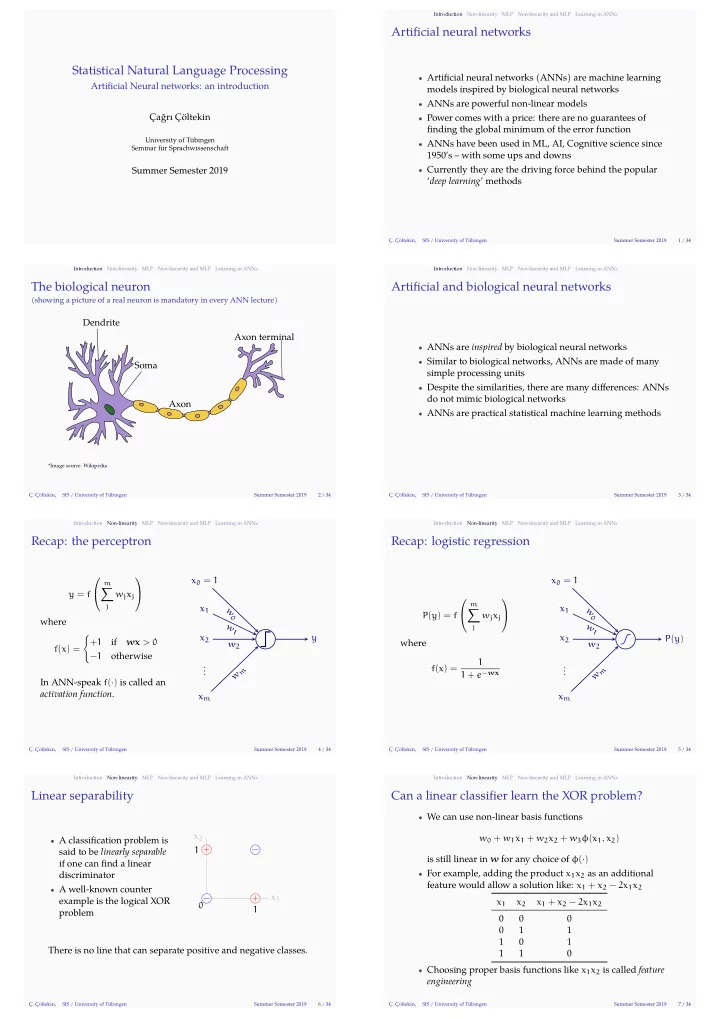
The biological neuron

(showing a picture of a real neuron is mandatory in every ANN lecture)

Axon terminal Axon Soma Dendrite

*Image source: Wikipedia Ç. Çöltekin, SfS / University of Tübingen Summer Semester 2019 2 / 34 Introduction Non-linearity MLP Non-linearity and MLP Learning in ANNs

Artifjcial and biological neural networks

• ANNs are inspired by biological neural networks
• Similar to biological networks, ANNs are made of many

simple processing units

• Despite the similarities, there are many difgerences: ANNs

do not mimic biological networks

• ANNs are practical statistical machine learning methods

Ç. Çöltekin, SfS / University of Tübingen Summer Semester 2019 3 / 34 Introduction Non-linearity MLP Non-linearity and MLP Learning in ANNs

Recap: the perceptron

y = f  

m

∑

j

wjxj   where f(x) = { +1 if wx > 0 −1

• therwise

In ANN-speak f(·) is called an activation function. x2 x1 . . . xm w1 w2 wm y x0 = 1 w0

Ç. Çöltekin, SfS / University of Tübingen Summer Semester 2019 4 / 34 Introduction Non-linearity MLP Non-linearity and MLP Learning in ANNs

Recap: logistic regression

P(y) = f  

m

∑

j

wjxj   where f(x) = 1 1 + e−wx x2 x1 . . . xm w1 w2 wm P(y) x0 = 1 w0

Ç. Çöltekin, SfS / University of Tübingen Summer Semester 2019 5 / 34 Introduction Non-linearity MLP Non-linearity and MLP Learning in ANNs

Linear separability

• A classifjcation problem is

said to be linearly separable if one can fjnd a linear discriminator

• A well-known counter

example is the logical XOR problem x2 x1 1 1 − + + − There is no line that can separate positive and negative classes.

Ç. Çöltekin, SfS / University of Tübingen Summer Semester 2019 6 / 34 Introduction Non-linearity MLP Non-linearity and MLP Learning in ANNs

Can a linear classifjer learn the XOR problem?

• We can use non-linear basis functions

w0 + w1x1 + w2x2 + w3φ(x1, x2) is still linear in w for any choice of φ(·)

• For example, adding the product x1x2 as an additional

feature would allow a solution like: x1 + x2 − 2x1x2 x1 x2 x1 + x2 − 2x1x2 1 1 1 1 1 1

• Choosing proper basis functions like x1x2 is called feature

engineering

Ç. Çöltekin, SfS / University of Tübingen Summer Semester 2019 7 / 34

SLIDE 2

Introduction Non-linearity MLP Non-linearity and MLP Learning in ANNs

Non-linear basis functions

solution in the original input space

1 1 − + + − x1 x2 The solution to x1 + x2 − 2x1x2 − 0.5 = 0 is a (non-linear) discriminant that solves the problem

Ç. Çöltekin, SfS / University of Tübingen Summer Semester 2019 8 / 34 Introduction Non-linearity MLP Non-linearity and MLP Learning in ANNs

Non-linear basis functions

solution in the 3D input space

1 1 0.5 1 x1 x2 x1x2

• The additional basis

function maps the problem into 3D

• In the new, mapped

space, the points are linearly separable

Ç. Çöltekin, SfS / University of Tübingen Summer Semester 2019 9 / 34 Introduction Non-linearity MLP Non-linearity and MLP Learning in ANNs

Where do non-linearities come from?

non-linearities are abundant in nature, it is not only the XOR problem

In a linear model, y = w0 + w1x1 + . . . + wkxk

• The outcome is linearly-related to the predictors
• The efgects of the inputs are additive

This is not always the case:

• Some predictors afgect the outcome in a non-linear way

– The efgect may be strong or positive only in a certain range

• f the variable (e.g., reaction time change by age)

– Some efgects are periodic (e.g., many measures of time)

• Some predictors interact

‘not bad’ is not ‘not’ + ‘bad’ (e.g., for sentiment analysis)

Ç. Çöltekin, SfS / University of Tübingen Summer Semester 2019 10 / 34 Introduction Non-linearity MLP Non-linearity and MLP Learning in ANNs

Multi-layer perceptron

• The simplest modern ANN architecture is called

multi-layer perceptron (MLP)

• The MLP is a fully connected, feed-forward network

consisting of perceptron-like units

• Unlike perceptron, the units in an MLP use a continuous

activation function

• The MLP can be trained using gradient-based methods
• The MLP can represent many interesting machine learning

problems

– It can be used for both regression and classifjcation

Ç. Çöltekin, SfS / University of Tübingen Summer Semester 2019 11 / 34 Introduction Non-linearity MLP Non-linearity and MLP Learning in ANNs

Multi-layer perceptron

the picture

x1 x2 x3 x4 y Input Hidden Output Each unit takes a weighted sum of their input, and applies a (non-linear) activation function.

Ç. Çöltekin, SfS / University of Tübingen Summer Semester 2019 12 / 34 Introduction Non-linearity MLP Non-linearity and MLP Learning in ANNs

Artifjcial neurons

∑ f(·) x2 x1 . . . xm w

1

w2 wm y x0 = 1 w0

• The unit calculates a

weighted sum of the inputs

m

∑

j

wjxj = wx

• Result is a linear

transformation

• Then the unit applies a

non-linear activation function f(·)

• Output of the unit is

y = f(wx)

Ç. Çöltekin, SfS / University of Tübingen Summer Semester 2019 13 / 34 Introduction Non-linearity MLP Non-linearity and MLP Learning in ANNs

Artifjcial neurons

an example

∑ x2 x1 . . . xm w

1

w2 wm y x0 = 1 w0

• A common activation

function is logistic sigmoid function f(x) = 1 1 + e−x

• The output of the network

becomes y = 1 1 + e−wx

Ç. Çöltekin, SfS / University of Tübingen Summer Semester 2019 14 / 34 Introduction Non-linearity MLP Non-linearity and MLP Learning in ANNs

Activation functions in ANNs

hidden units

• The activation functions in MLP are typically continuous

(difgerentiable) functions

• For hidden units common choices are

Sigmoid (logistic)

1 1+ex

Hyperbolic tangent (tanh)

e2x−1 e2x+1

Rectifjed linear unit (relu) max(0, x)

Ç. Çöltekin, SfS / University of Tübingen Summer Semester 2019 15 / 34

SLIDE 3

Introduction Non-linearity MLP Non-linearity and MLP Learning in ANNs

Activation functions in ANNs

• utput units
• The activation functions of the output units depends on

the task. Common choices are

– For regression, identity function – For binary classifjcation, logistic sigmoid P(y = 1 | x) = 1 1 + e−wx = ewx 1 + e−wx – For multi-class classifjcation, softmax P(y = k | x) = ewkx ∑

j ewjx

Ç. Çöltekin, SfS / University of Tübingen Summer Semester 2019 16 / 34 Introduction Non-linearity MLP Non-linearity and MLP Learning in ANNs

MLP: a simple example

x1 x2 h1 h2 y1 y2 f() g() w(1)

11

w(1)

12

w(1)

21

w(1)

22

w(2)

11

w(2)

21

w(2)

12

w(2)

22

hj = f (∑

i

w(1)

ij xi

) yk = g  ∑

j

w(2)

jk hj

  yk = g  ∑

j

w(2)

jk f

(∑

i

w(1)

ij xi

) 

Ç. Çöltekin, SfS / University of Tübingen Summer Semester 2019 17 / 34 Introduction Non-linearity MLP Non-linearity and MLP Learning in ANNs

MLP: a simple example

x1 x2 h1 h2 y1 y2 f() g() w(1)

11

w(1)

12

w(1)

21

w(1)

22

w(2)

11

w(2)

21

w(2)

12

w(2)

22

• Alternatively, we can write

the computations in matrix form h = f(W(1)x) y = g(W(2)h) = g ( W(2)f(W(1)x) )

• This corresponds to a

series of transformations followed by elementwise (non-linear) function applications

Ç. Çöltekin, SfS / University of Tübingen Summer Semester 2019 18 / 34 Introduction Non-linearity MLP Non-linearity and MLP Learning in ANNs

Solving non-linear problems with ANNs

a solution to XOR problem

x1 h1 y x2 h2

f(z) = z2 g(z) =

1 1+e−z

1 1

w

(1) 01

w

( 1 ) 2

w(2)

01

w

( 1 ) 1 1

w(1)

12

w(1)

21

w

( 1 ) 2 2

w(2)

11

w(2)

21

x2 x1 h2 h1 Is this difgerent from non-linear basis functions?

Ç. Çöltekin, SfS / University of Tübingen Summer Semester 2019 19 / 34 Introduction Non-linearity MLP Non-linearity and MLP Learning in ANNs

Solving non-linear problems with ANNs

a solution to XOR problem

4 0.27

f(z) = z2 g(z) =

1 1+e−z

1 1

− 2 3 1 1 1 1 −1 −1

x2 x1 h2 h1 Is this difgerent from non-linear basis functions?

Ç. Çöltekin, SfS / University of Tübingen Summer Semester 2019 19 / 34 Introduction Non-linearity MLP Non-linearity and MLP Learning in ANNs

Solving non-linear problems with ANNs

a solution to XOR problem

1 0.73 1 1

f(z) = z2 g(z) =

1 1+e−z

1 1

− 2 3 1 1 1 1 −1 −1

x2 x1 h2 h1 Is this difgerent from non-linear basis functions?

Ç. Çöltekin, SfS / University of Tübingen Summer Semester 2019 19 / 34 Introduction Non-linearity MLP Non-linearity and MLP Learning in ANNs

Solving non-linear problems with ANNs

a solution to XOR problem

1 1 0.73 1

f(z) = z2 g(z) =

1 1+e−z

1 1

− 2 3 1 1 1 1 −1 −1

x2 x1 h2 h1 Is this difgerent from non-linear basis functions?

Ç. Çöltekin, SfS / University of Tübingen Summer Semester 2019 19 / 34 Introduction Non-linearity MLP Non-linearity and MLP Learning in ANNs

Solving non-linear problems with ANNs

a solution to XOR problem

1 0.27 1 4

f(z) = z2 g(z) =

1 1+e−z

1 1

− 2 3 1 1 1 1 −1 −1

x2 x1 h2 h1 Is this difgerent from non-linear basis functions?

Ç. Çöltekin, SfS / University of Tübingen Summer Semester 2019 19 / 34

SLIDE 4

Introduction Non-linearity MLP Non-linearity and MLP Learning in ANNs

Non-linear activation functions are necessary

Without non-linear activation functions, an ANN with any number of layers is equivalent to a linear model. x1 h1 y x2 h2

a b c d e f

h1 = ax1 + cx2 h2 = bx1 + dx2 y = eh1 + fh2 = (ea + fb)x1 + (ec + fd)x2 y is still a linear function of xi

Ç. Çöltekin, SfS / University of Tübingen Summer Semester 2019 20 / 34 Introduction Non-linearity MLP Non-linearity and MLP Learning in ANNs

Gradient descent: a refresher

• The general idea is to approach a minimum of the error

function in small steps w ← w − η∇J(w)

– ∇J is the gradient of the loss function, it points to the direction of the maximum increase – η is the learning rate

• The updates can be performed

batch for the complete training set

• n-line after every training instance

– this is known as stochastic gradient descent (SGD) mini-batch after small fjxed-sized batches

Ç. Çöltekin, SfS / University of Tübingen Summer Semester 2019 21 / 34 Introduction Non-linearity MLP Non-linearity and MLP Learning in ANNs

Gradient descent: the picture

X ∇f(x1, . . . , xn) = ( ∂f ∂x1 , . . . , ∂f ∂xn ) A function is convex if there is only one (global) minimum.

Ç. Çöltekin, SfS / University of Tübingen Summer Semester 2019 22 / 34 Introduction Non-linearity MLP Non-linearity and MLP Learning in ANNs

Global and local minima

−20 20 −20 20 2 4 6

global min. local min. w1 w2 E(w)

Ç. Çöltekin, SfS / University of Tübingen Summer Semester 2019 23 / 34 Introduction Non-linearity MLP Non-linearity and MLP Learning in ANNs

Error functions in ANN training

depend on the task

• For regression, a natural choice is the minimizing the sum
• f squared error

E(w) = ∑

i

(yi − ˆ yi)2

• For binary classifjcation, we use cross entropy

E(w) = − ∑

i

yi log ˆ yi + (1 − yi) log(1 − ˆ yi)

• Similarly, for multi-class classifjcation, also cross entropy

E(w) = − ∑

i

∑

k

yi,k log ˆ yk In practice, the ANN loss functions will not be convex.

Ç. Çöltekin, SfS / University of Tübingen Summer Semester 2019 24 / 34 Introduction Non-linearity MLP Non-linearity and MLP Learning in ANNs

Learning in ANNs

• ANNs implement complex functions: we need to use
• ptimization methods (e.g., gradient descent) to train

them

• Typically error functions for ANNs are not convex,

gradient descent will fjnd a local minimum

• Optimization requires updating multiple layers of weights
• Assigning credit (or blame) to each weight during

learning is not trivial

• An efgective solution to the last problem is the

backpropagation algorithm

Ç. Çöltekin, SfS / University of Tübingen Summer Semester 2019 25 / 34 Introduction Non-linearity MLP Non-linearity and MLP Learning in ANNs

Learning in multi-layer networks: the problem

x1 x2 h1 h2 E(y) = ? y1 y2 E(y) = (y − ˆ y)2 f() g() w(1)

11

w(1)

12

w(1)

21

w(1)

22

w(2)

11

w(2)

21

w(2)

12

w(2)

22

We want a way to update non-fjnal weights based on fjnal error.

Ç. Çöltekin, SfS / University of Tübingen Summer Semester 2019 26 / 34 Introduction Non-linearity MLP Non-linearity and MLP Learning in ANNs

Calculating gradient on a neural network

(with some simplifjcation)

x1 h1 y x2 h2

E(w; y)

a b c d e f

• We need to calculate the gradient:

∇E = (∂E ∂a, ∂E ∂b, ∂E ∂c , ∂E ∂d, ∂E ∂e , ∂E ∂f ) we can use gradient descent directly

• ∂E

∂e and ∂E ∂f is easy, they do not

depend on other variables

• We factor others using chain rule

∂E ∂a = ∂h1 ∂a ∂E ∂h1 and ∂E ∂c = ∂h1 ∂c ∂E ∂h1

Ç. Çöltekin, SfS / University of Tübingen Summer Semester 2019 27 / 34

SLIDE 5

Introduction Non-linearity MLP Non-linearity and MLP Learning in ANNs

Backpropagation

x1 h1 y x2 h2

a b c d e f

• So far, it is just math

∂E ∂a = ∂h1 ∂a ∂E ∂h1 and ∂E ∂c = ∂h1 ∂c ∂E ∂h1

• But a naive implementation does

many repeated calculations

• Backpropagation is an effjcient

(dynamic programming) algorithm that avoids repeated calculations

• Backpropagation works for any

computation graph without cycles

Ç. Çöltekin, SfS / University of Tübingen Summer Semester 2019 28 / 34 Introduction Non-linearity MLP Non-linearity and MLP Learning in ANNs

Stochastic gradient descent

• Standard (batch) gradient

descent is computationally expensive: it updates weight at every epoch

• Stochastic gradient descent

(SGD) updates weights for every training instance

• SGD may take more steps, but

converges to the same solution w2 w1 error

• In practice a mini-batch is more common
• Correct batch size is not only about effjciency, it also afgects

accuracy

Ç. Çöltekin, SfS / University of Tübingen Summer Semester 2019 29 / 34 Introduction Non-linearity MLP Non-linearity and MLP Learning in ANNs

Preventing overfjtting in neural networks

• As in linear models, we can use L1 and L2 regularization

by adding a regularization term to the error function (known as weight decay). For example, J(w) = E(w) + ∥W∥

• There are other ways to fjght overfjtting

– With early stopping, one stops the training before it reaches to the smallest training error – With dropout, random units (with all of their connections) are dropped during training – Injecting noise at the output, as a way to (implicitly) model the noise in the target classes/values

Ç. Çöltekin, SfS / University of Tübingen Summer Semester 2019 30 / 34 Introduction Non-linearity MLP Non-linearity and MLP Learning in ANNs

Adapting learning rate

• The choice of learning rate η is important

too small slow convergence too big overshooting - may fmuctuate around the minimum,

• r even jump away
• The idea is to adapt the learning rate during learning
• A common trick is adding a momentum:

if we move in the same direction a long time accelerate ∆wij(t) = η ∂E ∂wij + α∆wij(t − 1)

• There are many adaptive optimization algorithms:

Adagrad, Adadelta, RMSprop, Adam, …

Ç. Çöltekin, SfS / University of Tübingen Summer Semester 2019 31 / 34 Introduction Non-linearity MLP Non-linearity and MLP Learning in ANNs

How many layers, units

• A network with single hidden layer is said to be a universal

approximator: it can approximate any continuous function with arbitrary precision

• However, in practice multiple interconnected layers are

useful and commonly used in modern ANN models

• The choice of layers, in general the architecture of the

system, depends on the application

Ç. Çöltekin, SfS / University of Tübingen Summer Semester 2019 32 / 34 Introduction Non-linearity MLP Non-linearity and MLP Learning in ANNs

A bit of history

1950-60 ANNs (perceptron) became popular: lots of excitement in AI, cognitive science 1970s Not much interest

– criticism on perceptron: linear separability

1980s ANNs became popular again

– backpropagation algorithm – multi-layer networks

1990s ANNs had again fallen ‘out of fashion’

– Engineering: other algorithms (such as SVMs) performed generally better – From the cognitive science perspective: ANNs are diffjcult to interpret

present ANNs (again) enjoy a renewed popularity with the name ‘deep learning’

Ç. Çöltekin, SfS / University of Tübingen Summer Semester 2019 33 / 34 Introduction Non-linearity MLP Non-linearity and MLP Learning in ANNs

Summary

• ANNs are powerful non-linear learners

– based on some inspiration from biological NNs – using many simple processing units – built on linear models (logistic regression)

• For non-linear problems we need non-linear activation

functions, and at least one hidden layer

• ANNs can be used for both regression and classifjcation
• ANN loss functions are not convex, what we fjnd is a local

minimum

• They (typically) are trained with backpropagation algorithm

Next: Mon/Fri Unsupervised learning

Ç. Çöltekin, SfS / University of Tübingen Summer Semester 2019 34 / 34

Additional reading, references, credits

• Third edition (draft) of Jurafsky and Martin, has a new

chapter on neural networks

• Hastie, Tibshirani, and Friedman (2009, ch.11) also

includes an accessible introduction

• For a reivew of use of ANNs in NLP, including more

advanced topics, see Goldberg 2016

Ç. Çöltekin, SfS / University of Tübingen Summer Semester 2019 A.1

SLIDE 6

Additional reading, references, credits (cont.)

Goldberg, Yoav (2016). “A primer on neural network models for natural language processing”. In: Journal of Artifjcial Intelligence Research 57, pp. 345–420. Hastie, Trevor, Robert Tibshirani, and Jerome Friedman (2009). The Elements of Statistical Learning: Data Mining, Inference, and Prediction. Second. Springer series in statistics. Springer-Verlag New York. isbn: 9780387848587. url: http://web.stanford.edu/~hastie/ElemStatLearn/. Jurafsky, Daniel and James H. Martin (2009). Speech and Language Processing: An Introduction to Natural Language Processing, Computational Linguistics, and Speech Recognition. second. Pearson Prentice Hall. isbn: 978-0-13-504196-3. Ç. Çöltekin, SfS / University of Tübingen Summer Semester 2019 A.2