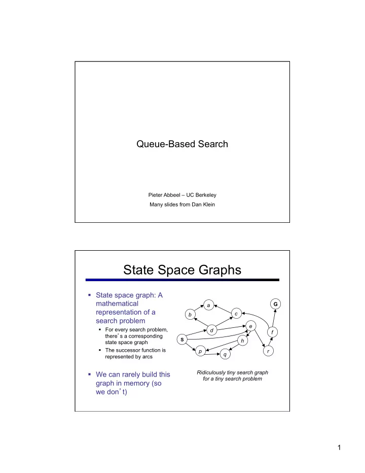
State Space Graphs State space graph: A mathematical G a - PDF document

Queue-Based Search Pieter Abbeel – UC Berkeley Many slides from Dan Klein State Space Graphs § State space graph: A mathematical G a representation of a c b search problem e § For every search problem, d f there ’ s a corresponding S h state space graph § The successor function is p r q represented by arcs Ridiculously tiny search graph § We can rarely build this for a tiny search problem graph in memory (so we don ’ t) 1

Search Trees “ N ” , 1.0 “ E ” , 1.0 § A search tree: § This is a “ what if ” tree of plans and outcomes § Start state at the root node § Children correspond to successors § Nodes contain states, correspond to PLANS to those states § For most problems, we can never actually build the whole tree Another Search Tree § Search: § Expand out possible plans § Maintain a fringe of unexpanded plans § Try to expand as few tree nodes as possible 2

General Tree Search § Important ideas: § Fringe § Expansion § Exploration strategy § Main question: which fringe nodes to explore? Example: Tree Search G a c b e d f S h p r q 3

State Graphs vs. Search Trees G a Each NODE in in the c search tree is an b entire PATH in the e d f problem graph. S h p r q S e p d q b c e h r We construct both on demand – and a a h r p q f we construct as little as possible. q c p q f G a q c G a Depth First Search G a a Strategy: expand c c b b deepest node first e e d d f f Implementation: S h h Fringe is a LIFO p p r r stack q q S e p d q b c e h r a a h r p q f q c p q f G a q c G a 4

Breadth First Search G a Strategy: expand c b shallowest node first e d Implementation: f S h Fringe is a FIFO queue p r q S e p d Search q b c e h r Tiers a a h r p q f q c p q f G a q c G a Costs on Actions GOAL a 2 2 c b 3 2 1 8 2 e d 3 f 9 8 2 START h 4 1 1 4 p r 15 q Notice that BFS finds the shortest path in terms of number of transitions. It does not find the least-cost path. We will quickly cover an algorithm which does find the least-cost path. 5

Uniform Cost Search 2 G a c b 8 1 Expand cheapest node first: 2 2 e 3 d Fringe is a priority queue f 8 1 9 S h 1 1 p r q 15 0 S 1 e 9 p 3 d 16 5 17 11 q 4 e h r b c 11 Cost 7 6 h 13 r p q f a a contours q c p q f 8 G a q c 11 10 G a Priority Queue Refresher § A priority queue is a data structure in which you can insert and retrieve (key, value) pairs with the following operations: pq.push(key, value) inserts (key, value) into the queue. returns the key with the lowest value, and pq.pop() removes it from the queue. § You can decrease a key ’ s priority by pushing it again § Unlike a regular queue, insertions aren ’ t constant time, usually O(log n ) § We ’ ll need priority queues for cost-sensitive search methods 6

Uniform Cost Issues § Remember: explores c ≤ 1 … increasing cost contours c ≤ 2 c ≤ 3 § The good: UCS is complete and optimal! § The bad: § Explores options in every “ direction ” § No information about goal location Start Goal Search Heuristics § Any estimate of how close a state is to a goal § Designed for a particular search problem § Examples: Manhattan distance, Euclidean distance 10 5 11.2 7

Heuristics Combining UCS and a Heuristic § Uniform-cost orders by path cost, or backward cost g(n) 5 h=1 e 1 1 3 2 S a d G h=6 h=5 1 h=2 h=0 1 c b h=7 h=6 § A* Search orders by the sum: f(n) = g(n) + h(n) Example: Teg Grenager 8

When should A* terminate? § Should we stop when we enqueue a goal? A 2 2 h = 2 G S h = 3 h = 0 B 3 2 h = 1 § No: only stop when we dequeue a goal Is A* Optimal? 1 A 3 h = 6 h = 0 S h = 7 G 5 § What went wrong? § Actual bad goal cost < estimated good goal cost § We need estimates to be less than actual costs! 9

Admissible Heuristics § A heuristic h is admissible (optimistic) if: where is the true cost to a nearest goal § Examples: 15 366 § Coming up with admissible heuristics is most of what ’ s involved in using A* in practice. Optimality of A*: Blocking Proof: … § What could go wrong? § We ’ d have to have to pop a suboptimal goal G off the fringe before G* § This can ’ t happen: § Imagine a suboptimal goal G is on the queue § Some node n which is a subpath of G* must also be on the fringe (why?) § n will be popped before G 10

UCS vs A* Contours § Uniform-cost expanded in all directions Start Goal § A* expands mainly toward the goal, but does hedge its bets to ensure optimality Start Goal Comparison Greedy Uniform Cost A star 11

Creating Admissible Heuristics § Most of the work in solving hard search problems optimally is in coming up with admissible heuristics § Often, admissible heuristics are solutions to relaxed problems, with new actions ( “ some cheating ” ) available 366 15 § Inadmissible heuristics are often useful too (why?) Example: 8 Puzzle § What are the states? § How many states? § What are the actions? § What states can I reach from the start state? § What should the costs be? 12

8 Puzzle I § Heuristic: Number of tiles misplaced § Why is it admissible? Average nodes expanded when 8 § h(start) = optimal path has length … … 4 steps … 8 steps … 12 steps § This is a relaxed- UCS 112 6,300 3.6 x 10 6 problem heuristic TILES 13 39 227 8 Puzzle II § What if we had an easier 8-puzzle where any tile could slide any direction at any time, ignoring other tiles? § Total Manhattan distance Average nodes expanded when § Why admissible? optimal path has length … … 4 steps … 8 steps … 12 steps § h(start) = 3 + 1 + 2 + … TILES 13 39 227 MANHATTAN 12 25 73 = 18 13

8 Puzzle III § How about using the actual cost as a heuristic? § Would it be admissible? § Would we save on nodes expanded? § What ’ s wrong with it? § With A*: a trade-off between quality of estimate and work per node! Tree Search: Extra Work! § Failure to detect repeated states can cause exponentially more work. Why? 14

287 Graph Search (~=188!) § Very simple fix: check if state worth expanding again: § Keep around “expanded list”, which stores pairs (expanded node, g-cost the expanded node was reached with) § When about to expand a node, only expand it if either (i) it has not been expanded before (in 188 lingo: are not in the closed list) or (ii) it has been expanded before, but the new way of reaching this node is cheaper than the cost it was reached with when expanded before § How about “consistency” of the heuristic function? § = condition on heuristic function § If heuristic is consistent, then the “new way of reaching the node” is guaranteed to be more expensive, hence a node never gets expanded twice; § In other words: if heuristic is consistent then when a node is expanded, the shortest path from the start state to that node has been found Consistency § Wait, how do we know parents have better f-vales than their successors? § Couldn ’ t we pop some node n , and find its child n ’ to have lower f value? § YES: h = 0 h = 8 B 3 g = 10 G A h = 10 § What can we require to prevent these inversions? § Consistency: § Real cost must always exceed reduction in heuristic 15

Optimality § Tree search: § A* optimal if heuristic is admissible (and non- negative) § UCS is a special case (h = 0) § 287 Graph search: § A* optimal if heuristic is admissible § A* expands every node only once if heuristic also consistent § UCS optimal (h = 0 is consistent) § Consistency implies admissibility § In general, natural admissible heuristics tend to be consistent Weighted A* f = g+ ε h § Weighted A*: expands states in the order of f = g+ ε h values, ε > 1 = bias towards states that are closer to goal 37 16

Weighted A* f = g+ ε h : ε = 0 --- Uniform Cost Search … … s start s goal University of Pennsylvania 38 Weighted A* f = g+ ε h : ε = 1 --- A* … … s start s goal 39 17

Weighted A* f = g+ ε h : ε > 1 … … s start s goal key to finding solution fast: shallow minima for h(s)-h*(s) function 40 Weighted A* f = g+ ε h : ε > 1 § Trades off optimality for speed § ε -suboptimal: § cost(solution) ≤ ε· cost(optimal solution) § Test your understanding by trying to prove this! § In many domains, it has been shown to be orders of magnitude faster than A* § Research becomes to develop a heuristic function that has shallow local minima 41 18