Stat 8053, Fall 2013: Robust Regression Duncans occupational-prestige - - PowerPoint PPT Presentation

Stat 8053, Fall 2013: Robust Regression

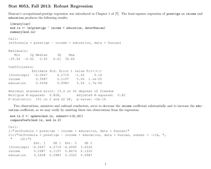
Duncan’s occupational-prestige regression was introduced in Chapter 1 of [?]. The least-squares regression of prestige on income and education produces the following results: library(car) mod.ls <- lm(prestige ~ income + education, data=Duncan) summary(mod.ls) Call: lm(formula = prestige ~ income + education, data = Duncan) Residuals: Min 1Q Median 3Q Max

• 29.54
• 6.42

0.65 6.61 34.64 Coefficients: Estimate Std. Error t value Pr(>|t|) (Intercept)

• 6.0647

4.2719

• 1.42

0.16 income 0.5987 0.1197 5.00 1.1e-05 education 0.5458 0.0983 5.56 1.7e-06 Residual standard error: 13.4 on 42 degrees of freedom Multiple R-squared: 0.828, Adjusted R-squared: 0.82 F-statistic: 101 on 2 and 42 DF, p-value: <2e-16 Two observations, ministers and railroad conductors, serve to decrease the income coefficient substantially and to increase the edu- cation coefficient, as we may verify by omitting these two observations from the regression: mod.ls.2 <- update(mod.ls, subset=-c(6,16)) compareCoefs(mod.ls, mod.ls.2) Call: 1:"lm(formula = prestige ~ income + education, data = Duncan)" 2:c("lm(formula = prestige ~ income + education, data = Duncan, subset = -c(6, ", " 16))")

• Est. 1

SE 1

• Est. 2

SE 2 (Intercept) -6.0647 4.2719 -6.4090 3.6526 income 0.5987 0.1197 0.8674 0.1220 education 0.5458 0.0983 0.3322 0.0987 1

Alternatively, let us compute the Huber M-estimator for Duncan’s regression model, using the rlm (robust linear model) function in the MASS library: library(MASS) mod.huber <- rlm(prestige ~ income + education, data=Duncan) summary(mod.huber) Call: rlm(formula = prestige ~ income + education, data = Duncan) Residuals: Min 1Q Median 3Q Max

• 30.12
• 6.89

1.29 4.59 38.60 Coefficients: Value

• Std. Error t value

(Intercept) -7.111 3.881

• 1.832

income 0.701 0.109 6.452 education 0.485 0.089 5.438 Residual standard error: 9.89 on 42 degrees of freedom The summary method for rlm objects prints the correlations among the coefficients; to suppress this output, specify correlation=FALSE. compareCoefs(mod.ls, mod.ls.2, mod.huber) Call: 1:"lm(formula = prestige ~ income + education, data = Duncan)" 2:c("lm(formula = prestige ~ income + education, data = Duncan, subset = -c(6, ", " 16))") 3:"rlm(formula = prestige ~ income + education, data = Duncan)"

• Est. 1

SE 1

• Est. 2

SE 2

• Est. 3

SE 3 (Intercept) -6.0647 4.2719 -6.4090 3.6526 -7.1107 3.8813 income 0.5987 0.1197 0.8674 0.1220 0.7014 0.1087 education 0.5458 0.0983 0.3322 0.0987 0.4854 0.0893 The Huber regression coefficients are between those produced by the least-squares fit to the full data set and by the least-squares fit eliminating the occupations minister and conductor. It is instructive to extract and plot (in Figure ??) the final weights used in the robust fit. The showLabels function from car is used to label all observations with weights less than 0.9. 2

plot(mod.huber$w, ylab="Huber Weight") bigweights <- which(mod.huber$w < 0.9) showLabels(1:45, mod.huber$w, rownames(Duncan), id.method=bigweights, cex.=.6) minister reporter conductor contractor 6 9 16 17 factory.owner mail.carrier insurance.agent store.clerk 18 22 23 24 machinist streetcar.motorman 28 33

• ● ● ● ●
• ●
• ● ● ● ● ●
• ●
• ● ●
• ●
• ● ●
• ● ● ● ● ● ● ● ● ● ● ●

10 20 30 40 0.4 0.5 0.6 0.7 0.8 0.9 1.0 Index Huber Weight minister reporter conductor contractor factory.owner mail.carrier insurance.agent store.clerk machinist streetcar.motorman

Ministers and conductors are among the observations that receive the smallest weight.

L1 Regression

We start by assuming a model like this: yi = x′

iβ + ei

(1) 3

where the e are random variables. We will estimate β by soling the minimization problem ˜ β = arg min 1 n

n

• i=1

|yi − x′

iβ| = 1

n

n

• i=1

ρ.5(yi − x′

iβ)

(2) where the objective function ρτ(u) is called in this instance a check function, ρτ(u) = u × (τ − I(u < 0)) (3) where I is the indicator function (more on check functions later). If the e are iid from a double exponential distribution, then ˜ β will be the corresponding mle for β. In general, however, we will be estimating the median at x′

iβ, so one can think of this as median regression.

Example We begin with a simple simulated example with n1 “good” observations and n2 “bad” ones. set.seed(10131986) library(MASS) library(quantreg) l1.data <- function(n1=100,n2=20){ data <- mvrnorm(n=n1,mu=c(0, 0), Sigma=matrix(c(1, .9, .9, 1), ncol=2)) # generate 20 ✬bad✬ observations data <- rbind(data, mvrnorm(n=n2, mu=c(1.5, -1.5), Sigma=.2*diag(c(1, 1)))) data <- data.frame(data) names(data) <- c("X", "Y") ind <- c(rep(1, n1),rep(2, n2)) plot(Y ~ X, data, pch=c(3, 20)[ind], col=c("black", "red")[ind], main=paste("N1 =",n1," N2 =", n2)) summary(r1 <-rq(Y ~ X, data=data, tau=0.5)) abline(r1) abline(lm(Y ~ X, data),lty=2, col="red") abline(lm(Y ~ X, data, subset=1:n1), lty=1, col="blue") legend("topleft", c("L1","ols","ols on good"), inset=0.02, lty=c(1, 2, 1), col=c("black", "red", "blue"), cex=.9)} par(mfrow=c(2, 2)) l1.data(100, 20) l1.data(100, 30) l1.data(100, 75) l1.data(100, 100) 4

• −2

−1 1 2 −2 −1 1 2

N1 = 100 N2 = 20

X Y

L1

• ls
• ls on good
• −2

−1 1 2 3 −3 −2 −1 1 2 3

N1 = 100 N2 = 30

X Y

L1

• ls
• ls on good
• −2

−1 1 2 3 −2 −1 1 2 3

N1 = 100 N2 = 75

X Y

L1

• ls
• ls on good
• −2

−1 1 2 −3 −2 −1 1 2

N1 = 100 N2 = 100

X Y

L1

• ls
• ls on good

5

Comparing L1 and L2

L1 minimizes the sum of the absolute errors while L2 minimizes squared errors. L1 gives much less weight to large deviations. Here are the ρ-functions for L1 and L2. curve(abs(x),-2,2,ylab="L1 or L2 or Huber M evaluated at x" ) curve(x^2,-3,3,add=T,col="red") abline(h=0) abline(v=0)

−2 −1 1 2 0.0 0.5 1.0 1.5 2.0 x L1 or L2 or Huber M evaluated at x Quantile regression

L1 is a special case of quantile regression in which we minimize the τ = .50-quantile, but a similar calculation can be done for any 0 < τ < 1. Here is what the check function (2) looks like for τ ∈ {.25, .5, .9}. rho <- function(u) { u * (tau - ifelse(u < 0,1,0) )} 6

tau <- .25; curve(rho,-2,2,lty=1) tau <- .50; curve(rho, -2,2,lty=2,col="blue",add=T,lwd=2) tau <- .90; curve(rho, -2,2,lty=3,col="red",add=T, lwd=3) abline(v=0,lty=5,col="gray") legend("bottomleft",c(".25",".5",".9"),lty=1:3,col=c("black","blue","red"),cex=.6) −2 −1 1 2 0.0 0.5 1.0 1.5 x rho(x)

.25 .5 .9

Quantile regression is just like L1 regression with ρτ replacing ρ.5 in (2), and with τ replacing 0.5 in the asymptotics.

• Example. This example shows expenditures on food as a function of income for nineteenth-century Belgian households.

data(engel) plot(foodexp~income,engel,cex=.5,xlab="Household Income", ylab="Food Expenditure", pch=20) abline(rq(foodexp~income,data=engel,tau=.5),col="blue") taus <- c(.1,.25,.75,.90) for( i in 1:length(taus)){ abline(rq(foodexp~income,data=engel,tau=taus[i]),col="gray") } 7

• ●
• 1000

2000 3000 4000 5000 500 1000 1500 2000 Household Income Food Expenditure

plot(summary(rq(foodexp~income,data=engel,tau=2:98/100))) 8

0.0 0.2 0.4 0.6 0.8 1.0 20 60 100 140

(Intercept)

• 0.0

0.2 0.4 0.6 0.8 1.0 0.3 0.5 0.7 0.9

income

• (The horizontal line is the ols estimate, with the dashed lines for confidence interval for it.)

Second Example This example examines salary as a function of job difficulty for job classes in a large governmental unit. Points are marked according to whether or not the fraction of female employees in the class exceeds 80%. library(alr4) mdom <- with(salarygov, NW/NE < .8) 9

taus <- c(.1, .5, .9) cols <- c("blue", "red", "blue") x <- 100:900 plot(MaxSalary ~ Score, salarygov, xlim=c(100, 1000), ylim=c(1000, 10000), cex=0.75, pch=c(20, 3)[mdom + 1]) for( i in 1:length(taus)){ lines(x, predict(rq(MaxSalary ~ bs(Score,5), data=salarygov[mdom, ], tau=taus[i]), newdata=data.frame(Score=x)), col=cols[i],lwd=2) } legend("topleft",paste("Quantile",taus),lty=1,col=cols,inset=.01, cex=.8) legend("bottomright",c("Female","Male"),pch=c(20, 3),inset=.01, cex=.8)

• 200

400 600 800 1000 2000 4000 6000 8000 10000 Score MaxSalary

Quantile 0.1 Quantile 0.5 Quantile 0.9

• Female

Male

10

plot(MaxSalary ~ Score, salarygov[!mdom, ], xlim=c(100, 1000), ylim=c(1000, 10000), cex=0.75, pch=20) for( i in 1:length(taus)){ lines(x, predict(rq(MaxSalary ~ bs(Score,5), data=salarygov[mdom, ], tau=taus[i]), newdata=data.frame(Score=x)), col=cols[i],lwd=2) } legend("topleft",paste("Quantile",taus),lty=1,col=cols,inset=.01, cex=.8) legend("bottomright",c("Female"),pch=c(20),inset=.01, cex=.8)

• 200

400 600 800 1000 2000 4000 6000 8000 10000 Score MaxSalary

Quantile 0.1 Quantile 0.5 Quantile 0.9

• Female

11