
SLIDE 1
STAR-CCM+: NACA0012 Flow and Aero-Acoustics Analysis James Ruiz - - PowerPoint PPT Presentation
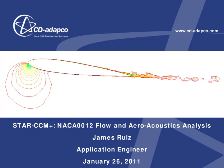
www.cd-adapco.com STAR-CCM+: NACA0012 Flow and Aero-Acoustics Analysis James Ruiz Application Engineer January 26, 2011 Introduction The objective of this work is to prove the capability of STAR-CCM+ as a Computational Fluid Dynamics
) ( * 2 3 2
3
Hz V k FMC =
] [ 00359 . 340 22 . 1 ] / [ ] [ tan ] [ s s m nd SpeedofSou m ce Dis s Time = = =
] [ 5 . 5 1286 . 4572 . log 10 log 10 ] [
10 10
dB L L dB SPL
Analysis Experiment
= = =
Man hrs: 0.5 Man hrs: 1.0 CPU hrs: 0.5 Man hrs: 1.0
Man hrs: 1.0
Cell count: 9.5M Inner Iterations: 15 Time Steps: 4000 Physical Time: 0.04 s CPU hrs: 89 (3.7 days)
Man hrs: 0.5