Spectral Estimation Overview Introduction Periodogram R x (e j - - PowerPoint PPT Presentation

spectral estimation overview introduction
SMART_READER_LITE
LIVE PREVIEW

Spectral Estimation Overview Introduction Periodogram R x (e j - - PowerPoint PPT Presentation

Spectral Estimation Overview Introduction Periodogram R x (e j ) r x ( )e j Bias, variance, and distribution l = Blackman-Tukey Method Most stationary random processes have continuous spectra


slide-1
SLIDE 1

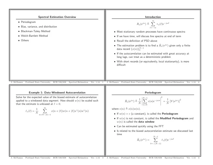
Example 1: Data Windowed Autocorrelation Solve for the expected value of the biased estimate of autocorrelation applied to a windowed data segment. How should w(n) be scaled such that the estimate is unbiased at ℓ = 0. ˆ rx(ℓ) = 1 N

  • n=N−|ℓ|−1

x(n + |ℓ|)w(n + |ℓ|)x∗(n)w∗(n)

  • J. McNames

Portland State University ECE 538/638 Spectral Estimation

  • Ver. 1.14

3

Spectral Estimation Overview

  • Periodogram
  • Bias, variance, and distribution
  • Blackman-Tukey Method
  • Welch-Bartlett Method
  • Others
  • J. McNames

Portland State University ECE 538/638 Spectral Estimation

  • Ver. 1.14

1

Periodogram ˆ Rx(ejω) 1 N

  • N−1
  • n=0

v(n)e−jωn

  • 2

= 1 N

  • V (ejω)
  • 2

where v(n) x(n)w(n).

  • If w(n) = c (a constant), is called the Periodogram
  • If w(n) is not constant, is called the Modified Periodogram and

w(n) is called the data window

  • Can be estimated quickly using the FFT
  • Is related to the biased autocorrelation estimate we discussed last

time ˆ Rx(ejω) =

N−1

  • ℓ=−(N−1)

ˆ rv(ℓ)e−jωℓ

  • J. McNames

Portland State University ECE 538/638 Spectral Estimation

  • Ver. 1.14

4

Introduction Rx(ejω)

  • l=−∞

rx(ℓ)e−jωℓ

  • Most stationary random processes have continuous spectra
  • If we have time, will discuss line spectra at end of term
  • Recall the definition of PSD above
  • The estimation problem is to find a ˆ

Rx(ejω) given only a finite data record {x(n)}N−1

  • If the autocorrelation can be estimated with great accuracy at

long lags, can treat as a deterministic problem

  • With short records (or equivalently, local stationarity), is more

difficult

  • J. McNames

Portland State University ECE 538/638 Spectral Estimation

  • Ver. 1.14

2

slide-2
SLIDE 2

Periodogram ˆ Rx(ejω) 1 N

  • N−1
  • n=0

v(n)e−jωn

  • 2

= 1 N

  • V (ejω)
  • 2 = F {ˆ

rv(ℓ)}

  • Remember that we must use the biased estimate of

autocorrelation – Otherwise the estimated PSD may be negative at some frequencies – The equality

1 N

  • V (ejω)
  • 2 = F {ˆ

rv(ℓ)} no longer holds

  • This relationship to ˆ

r(ℓ) means we can use the FFT to calculate ˆ r(ℓ) very efficiently – Take FFT of signal, magnitude square, and inverse FFT – Requires O(N log N) operations instead of O(N 2)! – Must take care to zero pad sufficiently

  • J. McNames

Portland State University ECE 538/638 Spectral Estimation

  • Ver. 1.14

7

Example 2: Periodogram and Biased Autocorrelation Let x(n) be a finite duration sequence, 0 to N − 1. Show that the biased estimate of autocorrelation is given by ˆ rx(ℓ) = 1 N x(ℓ) ∗ x(−ℓ) and that the DTFT of ˆ rx(ℓ) is equal to the Periodogram of x(n) when w(n) = 1.

  • J. McNames

Portland State University ECE 538/638 Spectral Estimation

  • Ver. 1.14

5

Example 3: Periodogram as a Filter Bank ˆ Rx(ejω) 1 N

  • N−1
  • n=0

v(n)e−jωn

  • 2
  • How is the periodogram a filter bank?
  • What is the transfer function of the filter?
  • How good are the filters? How close are they to ideal filters?
  • J. McNames

Portland State University ECE 538/638 Spectral Estimation

  • Ver. 1.14

8

Example 2: Workspace

  • J. McNames

Portland State University ECE 538/638 Spectral Estimation

  • Ver. 1.14

6

slide-3
SLIDE 3

Example 4: MATLAB Code

M = 500; % Padding to eliminate transient N = [25,50,100,250,500,1000]; % Length of signal segment NA = 500; % No. averages cb = 95; % Confidence Bands NZ = 1024; b = poly([-0.8,0.97*exp(j *pi/4),0.97*exp(-j *pi/4),... 0.97*exp(j *pi/6),0.97*exp(-j *pi/6)]); % Numerator a = poly([ 0.8,0.95*exp(j*3*pi/4),0.95*exp(-j*3*pi/4),... 0.95*exp(j*2.5*pi/4),0.95*exp(-j*2.5*pi/4)]); % Denominator b = b*sum(a)/sum(b); % Scale DC gain to 1

  • J. McNames

Portland State University ECE 538/638 Spectral Estimation

  • Ver. 1.14

11

Example 3: Work Space

  • J. McNames

Portland State University ECE 538/638 Spectral Estimation

  • Ver. 1.14

9

Example 4: Pole Zero Map of ARMA Process

−1 −0.5 0.5 1 −1 −0.5 0.5 1

  • J. McNames

Portland State University ECE 538/638 Spectral Estimation

  • Ver. 1.14

12

Example 4: Peridogram Generate the periodogram for a signal from a known LTI system with two sets of complex conjugate poles close to one another and near the unit circle. Repeat for various signal lengths.

  • J. McNames

Portland State University ECE 538/638 Spectral Estimation

  • Ver. 1.14

10

slide-4
SLIDE 4

Example 4: MATLAB Code

n = 100; w = randn(M+n,1); x = filter(b,a,w); % System with known PSD nx = length(x); x = x(nx-n+1:nx); % Eliminate start-up transient (make stationary) figure; k = 0:n-1; h = stem(k,x); set(h,’Marker’,’none’); set(h,’LineWidth’,0.5); box off; ylabel(’Signal’); xlabel(’Sample Index’); title(sprintf(’Length:%d’,n)); xlim([0 n]); ylim([min(x) max(x)]);

  • J. McNames

Portland State University ECE 538/638 Spectral Estimation

  • Ver. 1.14

15

Example 4: MATLAB Code

figure h = circle; z = roots(b); p = roots(a); hold on; h2 = plot(real(z),imag(z),’bo’,real(p),imag(p),’rx’); hold off; axis square; xlim([-1.1 1.1]); ylim([-1.1 1.1]); axislines; box off;

  • J. McNames

Portland State University ECE 538/638 Spectral Estimation

  • Ver. 1.14

13

Example 4: True PSD

0.05 0.1 0.15 0.2 0.25 0.3 0.35 0.4 0.45 0.5 1 2 3 x 10

5

PSD True PSD 0.05 0.1 0.15 0.2 0.25 0.3 0.35 0.4 0.45 0.5 10 PSD Frequency (cycles/sample)

  • J. McNames

Portland State University ECE 538/638 Spectral Estimation

  • Ver. 1.14

16

Example 4: Signal

10 20 30 40 50 60 70 80 90 100 −200 −100 100 200 300 Signal Sample Index Length:100

  • J. McNames

Portland State University ECE 538/638 Spectral Estimation

  • Ver. 1.14

14

slide-5
SLIDE 5

Example 4: Periodogram Estimate

0.05 0.1 0.15 0.2 0.25 0.3 0.35 0.4 0.45 0.5 1 2 3 4 x 10

5

PSD N:50 NA:1000 Confidence Bands:95% Single Estimate True PSD Confidence Bands Average Estimate 0.05 0.1 0.15 0.2 0.25 0.3 0.35 0.4 0.45 0.5 10 PSD Frequency (cycles/sample)

  • J. McNames

Portland State University ECE 538/638 Spectral Estimation

  • Ver. 1.14

19

Example 4: MATLAB Code

[R,w] = freqz(b,a,NZ); R2 = abs(R).^2; f = w/(2*pi); subplot(2,1,1); h = plot(f,R2,’r’); set(h,’LineWidth’,1.2); box off; ylabel(’PSD’); title(’True PSD’); xlim([0 0.5]); ylim([0 max(R2)*1.2]); subplot(2,1,2); h = semilogy(f,R2,’r’); set(h,’LineWidth’,1.2); box off; ylabel(’PSD’); xlim([0 0.5]); ylim([0.2*min(R2) max(R2)*5]); xlabel(’Frequency (cycles/sample)’);

  • J. McNames

Portland State University ECE 538/638 Spectral Estimation

  • Ver. 1.14

17

Example 4: Periodogram Estimate

0.05 0.1 0.15 0.2 0.25 0.3 0.35 0.4 0.45 0.5 1 2 3 4 x 10

5

PSD N:100 NA:1000 Confidence Bands:95% Single Estimate True PSD Confidence Bands Average Estimate 0.05 0.1 0.15 0.2 0.25 0.3 0.35 0.4 0.45 0.5 10 PSD Frequency (cycles/sample)

  • J. McNames

Portland State University ECE 538/638 Spectral Estimation

  • Ver. 1.14

20

Example 4: Periodogram Estimate

0.05 0.1 0.15 0.2 0.25 0.3 0.35 0.4 0.45 0.5 1 2 3 4 x 10

5

PSD N:25 NA:1000 Confidence Bands:95% Single Estimate True PSD Confidence Bands Average Estimate 0.05 0.1 0.15 0.2 0.25 0.3 0.35 0.4 0.45 0.5 10 PSD Frequency (cycles/sample)

  • J. McNames

Portland State University ECE 538/638 Spectral Estimation

  • Ver. 1.14

18

slide-6
SLIDE 6

Example 4: Periodogram Estimate

0.05 0.1 0.15 0.2 0.25 0.3 0.35 0.4 0.45 0.5 1 2 3 4 x 10

5

PSD N:1000 NA:1000 Confidence Bands:95% Single Estimate True PSD Confidence Bands Average Estimate 0.05 0.1 0.15 0.2 0.25 0.3 0.35 0.4 0.45 0.5 10 PSD Frequency (cycles/sample)

  • J. McNames

Portland State University ECE 538/638 Spectral Estimation

  • Ver. 1.14

23

Example 4: Periodogram Estimate

0.05 0.1 0.15 0.2 0.25 0.3 0.35 0.4 0.45 0.5 1 2 3 4 x 10

5

PSD N:250 NA:1000 Confidence Bands:95% Single Estimate True PSD Confidence Bands Average Estimate 0.05 0.1 0.15 0.2 0.25 0.3 0.35 0.4 0.45 0.5 10 PSD Frequency (cycles/sample)

  • J. McNames

Portland State University ECE 538/638 Spectral Estimation

  • Ver. 1.14

21

Example 4: MATLAB Code

for c1 = 1:length(N), nx = M+N(c1); Rh = zeros(NA,NZ/2+1); kh = 1:NZ/2+1; fh = (kh-1)/NZ; for c2 = 1:NA, w = randn(M+N(c1),1); x = filter(b,a,w); % System with known PSD x = x(nx-N(c1)+1:nx); % Eliminate start-up transient (make stationary) rh = (1/N(c1))*abs(fft(x,NZ)).^2; Rh(c2,:) = rh(kh).’; end; Rha = mean(Rh); % Average Rhu = prctile(Rh,100-(100-cb)/2); % Upper confidence band Rhl = prctile(Rh, (100-cb)/2); % Lower confidence band

  • J. McNames

Portland State University ECE 538/638 Spectral Estimation

  • Ver. 1.14

24

Example 4: Periodogram Estimate

0.05 0.1 0.15 0.2 0.25 0.3 0.35 0.4 0.45 0.5 1 2 3 4 x 10

5

PSD N:500 NA:1000 Confidence Bands:95% Single Estimate True PSD Confidence Bands Average Estimate 0.05 0.1 0.15 0.2 0.25 0.3 0.35 0.4 0.45 0.5 10 PSD Frequency (cycles/sample)

  • J. McNames

Portland State University ECE 538/638 Spectral Estimation

  • Ver. 1.14

22

slide-7
SLIDE 7

Periodogram Mean E

  • ˆ

Rx(ejω)

  • =

N−1

  • ℓ=−(N−1)

E [ˆ rv(ℓ)] e−jωℓ E [ˆ rv(ℓ)] = E

  • 1

N

  • n=−∞

x(n)w(n)x∗(n − ℓ)w∗(n − ℓ)

  • =

1 N

  • n=−∞

rx(ℓ)w(n)w∗(n − ℓ) = rx(ℓ) 1 N

  • n=−∞

w(n)w∗(n − ℓ) = 1 N rx(ℓ)rw(ℓ) The expected value of ˆ rv(ℓ) is the true autocorrelation rx(ℓ) windowed with rw(ℓ) = 1

N w(n) ∗ w(−n)∗.

  • J. McNames

Portland State University ECE 538/638 Spectral Estimation

  • Ver. 1.14

27

Example 4: MATLAB Code

figure; subplot(2,1,1); h = plot(fh,Rh(1,:),’g’,fh,Rhl,’b’,fh,Rhu,’b’,f,R2,’r’,fh,Rha,’k’); set(h(1) ,’LineWidth’,0.3); set(h(2:3),’LineWidth’,0.5); set(h(4) ,’LineWidth’,1.5); set(h(5) ,’LineWidth’,0.5); ylabel(’PSD’); title(sprintf(’N:%d NA:%d Confidence Bands:%d%%’,N(c1),NA,cb)); xlim([0 0.5]); ylim([0 max(R2)*1.5]); legend(h([1 2 4 5]),’Single Estimate’,’Confidence Bands’,’Average’,’True’,2); subplot(2,1,2); h = semilogy(fh,Rh(1,:),’g’,fh,Rhl,’b’,fh,Rhu,’b’,f,R2,’r’,fh,Rha,’k’); set(h(1) ,’LineWidth’,0.3); set(h(2:3),’LineWidth’,0.5); set(h(4) ,’LineWidth’,1.5); set(h(5) ,’LineWidth’,0.5); ylabel(’PSD’); xlabel(’Frequency (cycles/sample)’); xlim([0 0.5]); ylim([0.2*min(R2) max(R2)*5]); end;

  • J. McNames

Portland State University ECE 538/638 Spectral Estimation

  • Ver. 1.14

25

Periodogram Mean Continued E

  • ˆ

Rx(ejω)

  • =

N−1

  • ℓ=−(N−1)

E [ˆ rx(ℓ)] e−jωℓ = 1 N

N−1

  • ℓ=−(N−1)

rx(ℓ)rw(ℓ)e−jωℓ = 1 2π π

−π

Rx(eju) 1 N Rw

  • ej(ω−u)

du

  • Since E
  • ˆ

Rx(ejω)

  • = Rx(ejω), the Periodogram is a biased

estimator

  • Here Rw(ejω) = |W(ejω)|2 is the ESD of the window
  • Ideally, we would like Rw(ejω) = 2πNδ(ω)
  • The smearing limits our ability to distinguish sharp features (e.g.

distinct peaks) in the PSD

  • J. McNames

Portland State University ECE 538/638 Spectral Estimation

  • Ver. 1.14

28

Periodogram Properties

  • The main disadvantage of the Periodogram appears to be

excessive variance

  • As with any estimator, we would like to know the bias, variance,

covariance, confidence intervals, and distribution

  • We will consider these each in turn
  • J. McNames

Portland State University ECE 538/638 Spectral Estimation

  • Ver. 1.14

26

slide-8
SLIDE 8

Periodogram Covariance Theory ˆ Rw(ejω) = 1 N

  • N−1
  • n=0

w(n)ejωn

  • 2

= 1 N

  • N−1
  • n=0

w(n)ejk 2π

N n

  • 2
  • The text lists the covariance of the Periodogram, but does not

derive it

  • Details of the derivation can be found in [1]
  • An outline of the derivation is provided here
  • Suppose for now that no zero padding is used so we calculate the

DFT only at the N points that we have samples of the signal

  • Let w(n) be a WGN process with variance σ2

w and zero mean

  • J. McNames

Portland State University ECE 538/638 Spectral Estimation

  • Ver. 1.14

31

Periodogram Asymptotic Bias E

  • ˆ

Rx(ejω)

  • =

1 N

N−1

  • ℓ=−(N−1)

rx(ℓ)rw(ℓ)e−jωℓ

  • Most windows are relatively constant over a range of samples

proportional to the window length: rw(ℓ) ≈

  • N

|ℓ| ≪ N |ℓ| > N

  • Most stationary signals have an autocorrelation that approaches

zero as ℓ → ∞

  • Thus, the periodogram can be considered to be an asymptotically

unbiased estimator lim

N→∞ E

  • ˆ

Rx(ejω)

  • = Rx(ejω)
  • J. McNames

Portland State University ECE 538/638 Spectral Estimation

  • Ver. 1.14

29

Orthogonal Components Recall that when zero padding is not used, the exponentials are

  • rthogonal
  • n=<N>
  • ejk 2π

N n

ejℓ 2π

N n∗

=

  • n=<N>

ej(k−ℓ) 2π

N n

=

  • N

k = 0, ±N, ±2N, . . .

  • therwise

Now consider W(ejω) evaluated at ω = k 2π

N .

W(ejω) =

N−1

  • n=0

w(n)ejωn If w(n) is a WGN process, then W(ejω) is also a Gaussian random variable, since it is a linear combination of Gaussian RVs.

  • J. McNames

Portland State University ECE 538/638 Spectral Estimation

  • Ver. 1.14

32

Periodogram Asymptotic Bias Continued lim

N→∞ E

  • ˆ

Rx(ejω)

  • = Rx(ejω)
  • The estimator is unbiased as long as

N−1

  • n=0

|w(n)|2 = 1 2π π

−π

Rw(ejω) dω = N and the mainlobe window width decreases as

1 N

  • Not of much relevance (asymptotic result)
  • Practically, the bias is introduced by the sidelobes and smearing of

the spectrum by the main lobe

  • Can reduce with better windows, but can only trade main lobe

width for decreased sidebands

  • If signal is white noise (flat spectrum), the smearing of the

convolution does not cause bias

  • J. McNames

Portland State University ECE 538/638 Spectral Estimation

  • Ver. 1.14

30

slide-9
SLIDE 9

χ2 Random Variables

2 4 6 8 10 0.1 0.2 0.3 0.4 0.5 v=1 v=2 v=3 v=4 v=5 2 4 6 8 10 0.2 0.4 0.6 0.8 1 v=1 v=2 v=3 v=4 v=5

  • Let xi be a set of IID RVs with a Normal distribution,

xi ∼ N(0, 1)

  • Then the RV χ2 where

χ2 =

v

  • i=1

x2

i

has a χ2 distribution with v degrees of freedom

  • The PDF and CDF is available in MATLAB and equivalent
  • J. McNames

Portland State University ECE 538/638 Spectral Estimation

  • Ver. 1.14

35

WGN PSD Mean and Variance E

  • W(ejω)
  • =

N−1

  • n=0

E[w(n)]ejωn = 0 cov

  • W(ejω1), W(ejω2)
  • = E
  • W(ejω1)W(ejω2)∗

= E N−1

  • k=0

w(k)ejω1k N−1

  • ℓ=0

w(ℓ)ejω2ℓ ∗ =

N−1

  • k=0

N−1

  • ℓ=0

E[w(k)w(ℓ)∗]ejω1ke−jω2ℓ =

N−1

  • k=0

N−1

  • ℓ=0

σ2

wδ(k − ℓ)ej(ω1k−ω2ℓ)

= σ2

w N−1

  • k=0

ej(ω1−ω2)k

  • J. McNames

Portland State University ECE 538/638 Spectral Estimation

  • Ver. 1.14

33

MATLAB Code

x = linspace(0,10,100)’; df = 1:5; % Degrees of freedom nd = length(df); nx = length(x); P = zeros(nx,nd); C = zeros(nx,nd); for c1=1:5, P(:,c1) = chi2pdf(x,df(c1)); C(:,c1) = chi2cdf(x,df(c1)); ls{c1} = sprintf(’v=%d’,df(c1)); end; figure h = plot(x,P); set(h,’LineWidth’,1.5); box off; xlim([0 x(end)]); ylim([0 .5]); legend(ls); figure h = plot(x,C); set(h,’LineWidth’,1.5); box off; xlim([0 x(end)]); ylim([0 1.05]); legend(ls);

  • J. McNames

Portland State University ECE 538/638 Spectral Estimation

  • Ver. 1.14

36

WGN DFT Mean and Variance Continued If we don’t use zero padding, ω1 = m1 2π N ω2 = m2 2π N where m1 and m2 are integers. Then cov

  • W(ejω1), W(ejω2)
  • = σ2

w N−1

  • k=0

ej(ω1−ω2)k = σ2

w N−1

  • k=0

ej(m1−m2) 2π

N k

= σ2

wNδ(m1 − m2)

Thus, for WGN and no zero padding, the random variables are uncorrelated and therefore independent! The variance of the RVs is σ2

  • w. Alternative, the number of uncorrelated estimates in the frequency

domain scales with N. More data → more uncorrelated samples.

  • J. McNames

Portland State University ECE 538/638 Spectral Estimation

  • Ver. 1.14

34

slide-10
SLIDE 10

Generalized Linear Processes x(n) = h(n) ∗ w(n) =

  • k=−∞

h(k)w(n − k) Rx(ejω) = |H(ejω)|2σ2

w

  • This is a standard and widely used model for wide-sense stationary

processes

  • Note that h(n) is two sided (non-causal)
  • We require that h(n) has finite energy (a sufficient condition for

stability)

  • But how is ˆ

Rx(ejω) related to the known distribution of ˆ Rw(ejω)?

  • J. McNames

Portland State University ECE 538/638 Spectral Estimation

  • Ver. 1.14

39

WGN PSD Mean and Variance Continued E

  • W(ejω)
  • =

N−1

  • n=0

E[w(n)]ejωn = 0 cov

  • W(ejω1), W(ejω2)
  • = σ2

wNδ(ω1 − ω2)

ˆ Rw(ejω) = 1 N |W(ejω)|2

  • If W(ejω) is a complex Gaussian RV with zero mean and variance

σ2

w, then what is the distribution of |W(ejω)|2?

E

  • |W(ejω)|2]
  • = E
  • Re{W(ejω)}2 + Im{W(ejω)}2

= σ2

w

where the real and imaginary components are both independent Gaussian RVs each with variance σ2

w/2

  • Note that Im{W(ejω)} = 0 if ω = 0 or ω = π
  • J. McNames

Portland State University ECE 538/638 Spectral Estimation

  • Ver. 1.14

37

Periodogram Distribution It’s beyond the scope of this class to prove it (see [1, pg. 424]), but ˆ Rx(ejω) = Rx(ejω) 1 σ2

w

ˆ Rw(ejω) + Rε(ω) where E [Rε(ω)] = O(1/N 2)

  • Thus Rε(ω) → 0 as N → ∞
  • If we assume N is “large” we can disregard it

– N must be large enough to make the bias due to windowing negligible

  • This means that the periodogram estimate is χ2 distributed when

the process is Gaussian

  • We can then immediately write the distribution of ˆ

Rx(ejω)

  • J. McNames

Portland State University ECE 538/638 Spectral Estimation

  • Ver. 1.14

40

WGN PSD Distribution Thus the distribution of |W(ejω)|2 is given by |W(ejω)|2 σ2

wN

  • χ2(2)/2

ω = ℓπ χ2(1) ω = ℓπ where χ2(1) is a chi-squared distribution with one degree of freedom. Thus ˆ Rw(ejω) ∼

  • σwχ2(2)/2

ω = ℓπ σwχ2(1) ω = ℓπ Thus, we know what the distribution of ˆ Rw(ejω) is in the WGN case, but what about non-white processes?

  • J. McNames

Portland State University ECE 538/638 Spectral Estimation

  • Ver. 1.14

38

slide-11
SLIDE 11

Periodogram Variance (Again) var{ ˆ Rx(ejω)} ≈ R2

x(ejω)

  • 1 +

sin(ωN) N sin(ω) 2 For large N this can be approximated as var

  • ˆ

Rx(ejω)

  • R2

x(ejω)

0 < ω < π 2R2

x(ejω)

ω = 0, π

  • The variance depends on the true spectrum
  • Perhaps not surprising since the variance of ˆ

r(ℓ) depended on the true autocorrelation

  • Note that the variance does not decrease as N → ∞
  • Thus, the Periodogram is not a consistent estimator
  • The estimate becomes more variable as a function of frequency,

but the variance at a fixed frequency does not decrease

  • J. McNames

Portland State University ECE 538/638 Spectral Estimation

  • Ver. 1.14

43

Periodogram Distribution ˆ Rx(ejω) ∼

  • Rx(ejω)χ2(2)/2

ω = ℓπ Rx(ejω)χ2(1) ω = ℓπ Since var

  • χ2(2)/2
  • = 1

var

  • χ2(1)
  • = 2

The variance of the periodogram is given by var{ ˆ Rx(ejω)} ≈

  • R2

x(ejω)

0 < ω < π 2R2

x(ejω)

ω = 0, π which agrees with the text.

  • J. McNames

Portland State University ECE 538/638 Spectral Estimation

  • Ver. 1.14

41

Example 4: Periodogram Variance

0.05 0.1 0.15 0.2 0.25 0.3 0.35 0.4 0.45 0.5 5 10 x 10

10

var[PSD] N:25 NA:1000 Confidence Bands:95% Estimated Variance Theoretical Variance 0.05 0.1 0.15 0.2 0.25 0.3 0.35 0.4 0.45 0.5 10 var[PSD] Frequency (cycles/sample)

  • J. McNames

Portland State University ECE 538/638 Spectral Estimation

  • Ver. 1.14

44

Periodogram Covariance

  • Depends on the true, unknown PSD so is of limited value
  • Can make some qualitative observations
  • Estimates at two frequencies ω1 = (2π/N)k1 and ω2 = (2π/N)k2

where k1 and k2 are integers are approximately uncorrelated cov{ ˆ Rx(ejω1), ˆ Rx(ejω2)} ≈ 0 for k1 = k2

  • The number of uncorrelated frequency pairs scales with N
  • Thus, the periodogram at adjacent frequencies, say ω and ω + δ,

becomes more variable as N increases

  • J. McNames

Portland State University ECE 538/638 Spectral Estimation

  • Ver. 1.14

42

slide-12
SLIDE 12

Example 4: Periodogram Variance

0.05 0.1 0.15 0.2 0.25 0.3 0.35 0.4 0.45 0.5 5 10 x 10

10

var[PSD] N:250 NA:1000 Confidence Bands:95% Estimated Variance Theoretical Variance 0.05 0.1 0.15 0.2 0.25 0.3 0.35 0.4 0.45 0.5 10 var[PSD] Frequency (cycles/sample)

  • J. McNames

Portland State University ECE 538/638 Spectral Estimation

  • Ver. 1.14

47

Example 4: Periodogram Variance

0.05 0.1 0.15 0.2 0.25 0.3 0.35 0.4 0.45 0.5 5 10 x 10

10

var[PSD] N:50 NA:1000 Confidence Bands:95% Estimated Variance Theoretical Variance 0.05 0.1 0.15 0.2 0.25 0.3 0.35 0.4 0.45 0.5 10 var[PSD] Frequency (cycles/sample)

  • J. McNames

Portland State University ECE 538/638 Spectral Estimation

  • Ver. 1.14

45

Example 4: Periodogram Variance

0.05 0.1 0.15 0.2 0.25 0.3 0.35 0.4 0.45 0.5 5 10 x 10

10

var[PSD] N:500 NA:1000 Confidence Bands:95% Estimated Variance Theoretical Variance 0.05 0.1 0.15 0.2 0.25 0.3 0.35 0.4 0.45 0.5 10 var[PSD] Frequency (cycles/sample)

  • J. McNames

Portland State University ECE 538/638 Spectral Estimation

  • Ver. 1.14

48

Example 4: Periodogram Variance

0.05 0.1 0.15 0.2 0.25 0.3 0.35 0.4 0.45 0.5 5 10 x 10

10

var[PSD] N:100 NA:1000 Confidence Bands:95% Estimated Variance Theoretical Variance 0.05 0.1 0.15 0.2 0.25 0.3 0.35 0.4 0.45 0.5 10 var[PSD] Frequency (cycles/sample)

  • J. McNames

Portland State University ECE 538/638 Spectral Estimation

  • Ver. 1.14

46

slide-13
SLIDE 13

Fixing Problems with the Periodogram

  • As N increases, the ensemble variation stays constant

– The estimator is not consistent (statistically)

  • As N increases, the covariation at neighboring frequencies, ω and

ω + δ, decreases

  • Thus we are essentially able to estimate the true PSD at more

frequencies

  • We have better frequency resolution as N increases
  • Key assumption: the true PSD is smooth

– Clearly true for all ARMA processes with poles and zeros not too close to the unit circle

  • Key concept: If the PSD is smooth and our estimate consists of

uncorrelated high-resolution estimates, we can obtain a better estimate by averaging estimates at adjacent frequencies

  • J. McNames

Portland State University ECE 538/638 Spectral Estimation

  • Ver. 1.14

51

Example 4: Periodogram Variance

0.05 0.1 0.15 0.2 0.25 0.3 0.35 0.4 0.45 0.5 5 10 x 10

10

var[PSD] N:1000 NA:1000 Confidence Bands:95% Estimated Variance Theoretical Variance 0.05 0.1 0.15 0.2 0.25 0.3 0.35 0.4 0.45 0.5 10 var[PSD] Frequency (cycles/sample)

  • J. McNames

Portland State University ECE 538/638 Spectral Estimation

  • Ver. 1.14

49

Periodogram Smoothing

  • Smoothing the Periodogram can be thought of in several ways

– It reduces the frequency resolution – It blurs the spectrum – It increases the bias of the estimator – It reduces the variance of the estimator – It could either increase or decrease the MSE depending on the degree of smoothing and the variability of the true PSD

  • Thus, we can tradeoff some of the excessive variance of the

Periodogram for increases bias by smoothing

  • There are several ways to achieve this

– Average contiguous values of the periodogram – Average periodograms obtained from multiple segments

  • Both approaches produce about the same quality of estimators
  • J. McNames

Portland State University ECE 538/638 Spectral Estimation

  • Ver. 1.14

52

Periodogram Variance ˆ Rx(ejω) 1 N

  • N−1
  • n=0

v(n)e−jωn

  • 2

= 1 N

  • V (ejω)
  • 2 = F {ˆ

r(ℓ)}

  • Since the ensemble variance of the Periodogram does not decrease

as N increases, it is considered a poor estimator

  • We cannot fix this by choosing a better window
  • This is perhaps surprising, because it is the “natural” estimator
  • To obtain a better estimator, we need to reduce the ensemble

variance

  • J. McNames

Portland State University ECE 538/638 Spectral Estimation

  • Ver. 1.14

50

slide-14
SLIDE 14

Example 5: Smoothed Periodogram Estimate

0.05 0.1 0.15 0.2 0.25 0.3 0.35 0.4 0.45 0.5 1 2 3 4 x 10

5

PSD M:21 N:500 NA:1000 Confidence Bands:95% Single Estimate True PSD Confidence Bands Average Estimate 0.05 0.1 0.15 0.2 0.25 0.3 0.35 0.4 0.45 0.5 10 PSD Frequency (cycles/sample)

  • J. McNames

Portland State University ECE 538/638 Spectral Estimation

  • Ver. 1.14

55

Smoothing the Periodogram ˆ R(PS)

x

(ejωk) 1 2M + 1

M

  • j=−M

ˆ Rx(ejωk−j)

  • One approach to smoothing is to apply a moving average filter in

the frequency domain

  • In the definition above (borrowed from the book), only applies if

ˆ Rx(ejω) is known at discrete frequencies ωk (2π/N)k

  • This is usually the case because we estimate using the FFT
  • Since the examples at these discrete frequencies are approximately

uncorrelated var{ ˆ R(PS)

x

(ejωk)} ≈ 1 2M + 1 var{ ˆ Rx(ejωk)}

  • However, we increase the bias, especially near sharp features in the

frequency domain

  • J. McNames

Portland State University ECE 538/638 Spectral Estimation

  • Ver. 1.14

53

Example 5: Smoothed Periodogram Estimate

0.05 0.1 0.15 0.2 0.25 0.3 0.35 0.4 0.45 0.5 1 2 3 4 x 10

5

PSD M:51 N:500 NA:1000 Confidence Bands:95% Single Estimate True PSD Confidence Bands Average Estimate 0.05 0.1 0.15 0.2 0.25 0.3 0.35 0.4 0.45 0.5 10 PSD Frequency (cycles/sample)

  • J. McNames

Portland State University ECE 538/638 Spectral Estimation

  • Ver. 1.14

56

Example 5: Smoothed Periodogram Estimate

0.05 0.1 0.15 0.2 0.25 0.3 0.35 0.4 0.45 0.5 1 2 3 4 x 10

5

PSD M:11 N:500 NA:1000 Confidence Bands:95% Single Estimate True PSD Confidence Bands Average Estimate 0.05 0.1 0.15 0.2 0.25 0.3 0.35 0.4 0.45 0.5 10 PSD Frequency (cycles/sample)

  • J. McNames

Portland State University ECE 538/638 Spectral Estimation

  • Ver. 1.14

54

slide-15
SLIDE 15

Example 5: MATLAB Code Continued

for c1 = 1:length(Q), nx = P+N; Rh = zeros(NA,NZ/2+1); kh = 1:NZ/2+1; fh = (kh-1)/NZ; for c2 = 1:NA, w = randn(P+N,1); x = filter(b,a,w); % System with known PSD x = x(nx-N+1:nx); % Eliminate transient (make stationary) rh = (1/N)*abs(fft(x,NZ)).^2; rh = [rh;rh;rh]; % Eliminate edge effects rhs = filter(ones(Q(c1),1)/Q(c1),1,rh); rhs = rhs((Q(c1)-1)/2+(NZ+1:2*NZ)); % Account for filter delay Rh(c2,:) = rhs(kh).’; end; Rha = mean(Rh); % Average Rhu = prctile(Rh,100-(100-cb)/2); % Upper confidence band Rhl = prctile(Rh, (100-cb)/2); % Lower confidence band

  • J. McNames

Portland State University ECE 538/638 Spectral Estimation

  • Ver. 1.14

59

Example 5: Smoothed Periodogram Estimate

0.05 0.1 0.15 0.2 0.25 0.3 0.35 0.4 0.45 0.5 1 2 3 4 x 10

5

PSD M:101 N:500 NA:1000 Confidence Bands:95% Single Estimate True PSD Confidence Bands Average Estimate 0.05 0.1 0.15 0.2 0.25 0.3 0.35 0.4 0.45 0.5 10 PSD Frequency (cycles/sample)

  • J. McNames

Portland State University ECE 538/638 Spectral Estimation

  • Ver. 1.14

57

Example 5: MATLAB Code Continued

figure; FigureSet(1,’LTX’); subplot(2,1,1); h = plot(fh,Rh(1,:),’g’,f,R2,’r’,fh,Rhl,’b’,fh,Rhu,’b’,fh,Rha,’k’); set(h(1) ,’LineWidth’,0.3); set(h(2) ,’LineWidth’,1.3); set(h(3:4),’LineWidth’,0.5); set(h(5) ,’LineWidth’,0.5); ylabel(’PSD’); title(sprintf(’Q:%d N:%d NA:%d Confidence Bands:%d%%’,Q(c1),N,NA,cb)); xlim([0 0.5]); ylim([0 max(R2)*1.5]); legend(h([1 2 4 5]),’Single Estimate’,’Confidence Bands’,’Average’,’True’,2); subplot(2,1,2); h = semilogy(fh,Rh(1,:),’g’,f,R2,’r’,fh,Rhl,’b’,fh,Rhu,’b’,fh,Rha,’k’); set(h(1) ,’LineWidth’,0.3); set(h(2) ,’LineWidth’,1.3); set(h(3:4),’LineWidth’,0.5); set(h(5) ,’LineWidth’,0.5); ylabel(’PSD’); xlabel(’Frequency (cycles/sample)’); xlim([0 0.5]); ylim([0.2*min(R2) max(R2)*5]); end;

  • J. McNames

Portland State University ECE 538/638 Spectral Estimation

  • Ver. 1.14

60

Example 5: MATLAB Code

Q = [11,21,51,101]; % MA filter order N = 500; % Length of signal segment NA = 1000; % No. averages P = 500; % Padding to eliminate transient cb = 95; % Confidence Bands NZ = 2048; b = poly([-0.8,0.97*exp(j *pi/4),0.97*exp(-j *pi/4),... 0.97*exp(j *pi/6),0.97*exp(-j *pi/6)]); % Numerator a = poly([ 0.8,0.95*exp(j*3*pi/4),0.95*exp(-j*3*pi/4),... 0.95*exp(j*2.5*pi/4),0.95*exp(-j*2.5*pi/4)]); % Denominator b = b*sum(a)/sum(b); % Set DC gain to 1 [R,w] = freqz(b,a,NZ); R2 = abs(R).^2; f = w/(2*pi);

  • J. McNames

Portland State University ECE 538/638 Spectral Estimation

  • Ver. 1.14

58

slide-16
SLIDE 16

Blackman-Tukey Spectral Estimation ˆ R(BT)

x

(ejω)

L−1

  • ℓ=−(L−1)

ˆ rx(ℓ)wa(ℓ)e−jωℓ

  • Here the window is user specified and has a finite duration of

2L − 1 samples

  • Called the correlation or lag window
  • In order for the estimate to be nonnegative, W(ejω) ≥ 0 for all ω
  • Not all of the windows we described have this property
  • In the frequency domain, the product ˆ

rx(ℓ)w(ℓ) is equivalent to convolving with W(ejω)

  • Assuming the window’s spectrum is bumped shape, this

convolution smooths the spectrum

  • Note that the FFT can be used to calculate both ˆ

rx(ℓ) and ˆ R(BT)

x

(ejω) efficiently

  • J. McNames

Portland State University ECE 538/638 Spectral Estimation

  • Ver. 1.14

63

Periodogram Smoothing Comments ˆ R(PS)

x

(ejωk) 1 2M + 1

M

  • j=−M

ˆ Rx(ejωk−j) var

  • R(PS)

x

(ejω)

1 2M + 1 var

  • Rx(ejω)
  • Smoothing the periodogram is a good idea
  • Trades reduced frequency resolution and increased bias for

reduced variance

  • The moving average is just a lowpass filter
  • There are many other lowpass filters that might perform better
  • Examples: smoothing splines, local polynomial models, weighted

averaging (kernel smoothing)

  • J. McNames

Portland State University ECE 538/638 Spectral Estimation

  • Ver. 1.14

61

Blackman-Tukey Bias & Variance ˆ R(BT)

x

(ejω)

L−1

  • ℓ=−(L−1)

ˆ rx(ℓ)wa(ℓ)e−jωℓ

  • Conceptually, this is using an even more biased estimate of the

autocorrelation: ˆ rx(ℓ)wa(ℓ)

  • The additional bias is towards zero
  • Thus, it reduces the variance of both ˆ

rx(ℓ) and ˆ R(BT)

x

(ejω)

  • The user controls this tradeoff by picking the correlation window

wa(ℓ)

  • The window can be any positive definite window with even

symmetry (why?)

  • The length of the window L has a larger impact than the shape
  • J. McNames

Portland State University ECE 538/638 Spectral Estimation

  • Ver. 1.14

64

Blackman-Tukey Spectral Estimation Idea E

  • ˆ

Rx(ejω)

  • =

1 2π π

−π

Rx(eju) 1 N Rw(ej(ω−u)) du

  • Recall that windowing the signal is equivalent to convolving the

signal’s PSD with the window’s PSD, in expectation

  • Despite the blurring and smoothing of this effect, the estimate is

still has too high of variance

  • We can increase the smoothing and reduce the variance by

multiplying the autocorrelation by an even shorter window

  • J. McNames

Portland State University ECE 538/638 Spectral Estimation

  • Ver. 1.14

62

slide-17
SLIDE 17

Example 7: Blackman-Tukey Estimate

0.05 0.1 0.15 0.2 0.25 0.3 0.35 0.4 0.45 0.5 1 2 3 4 x 10

5

PSD N:500 L:51 NA:100 Confidence Bands:95% Single Estimate Average Estimated CIs True PSD Confidence Bands Average Estimate 0.05 0.1 0.15 0.2 0.25 0.3 0.35 0.4 0.45 0.5 10 PSD Frequency (cycles/sample)

  • J. McNames

Portland State University ECE 538/638 Spectral Estimation

  • Ver. 1.14

67

Example 6: Blackman-Tukey Estimate

0.05 0.1 0.15 0.2 0.25 0.3 0.35 0.4 0.45 0.5 1 2 3 4 x 10

5

PSD N:500 L:25 NA:100 Confidence Bands:95% Single Estimate Average Estimated CIs True PSD Confidence Bands Average Estimate 0.05 0.1 0.15 0.2 0.25 0.3 0.35 0.4 0.45 0.5 10 PSD Frequency (cycles/sample)

  • J. McNames

Portland State University ECE 538/638 Spectral Estimation

  • Ver. 1.14

65

Example 8: Blackman-Tukey Coverage

0.05 0.1 0.15 0.2 0.25 0.3 0.35 0.4 0.45 0.5 0.2 0.4 0.6 0.8 1 Coverage N:500 L:51 NA:100 Confidence Bands:95%

  • J. McNames

Portland State University ECE 538/638 Spectral Estimation

  • Ver. 1.14

68

Example 7: Blackman-Tukey Coverage

0.05 0.1 0.15 0.2 0.25 0.3 0.35 0.4 0.45 0.5 0.2 0.4 0.6 0.8 1 Coverage N:500 L:25 NA:100 Confidence Bands:95%

  • J. McNames

Portland State University ECE 538/638 Spectral Estimation

  • Ver. 1.14

66

slide-18
SLIDE 18

Example 9: Blackman-Tukey Estimate

0.05 0.1 0.15 0.2 0.25 0.3 0.35 0.4 0.45 0.5 1 2 3 4 x 10

5

PSD N:500 L:251 NA:100 Confidence Bands:95% Single Estimate Average Estimated CIs True PSD Confidence Bands Average Estimate 0.05 0.1 0.15 0.2 0.25 0.3 0.35 0.4 0.45 0.5 10 PSD Frequency (cycles/sample)

  • J. McNames

Portland State University ECE 538/638 Spectral Estimation

  • Ver. 1.14

71

Example 8: Blackman-Tukey Estimate

0.05 0.1 0.15 0.2 0.25 0.3 0.35 0.4 0.45 0.5 1 2 3 4 x 10

5

PSD N:500 L:101 NA:100 Confidence Bands:95% Single Estimate Average Estimated CIs True PSD Confidence Bands Average Estimate 0.05 0.1 0.15 0.2 0.25 0.3 0.35 0.4 0.45 0.5 10 PSD Frequency (cycles/sample)

  • J. McNames

Portland State University ECE 538/638 Spectral Estimation

  • Ver. 1.14

69

Example 10: Blackman-Tukey Coverage

0.05 0.1 0.15 0.2 0.25 0.3 0.35 0.4 0.45 0.5 0.2 0.4 0.6 0.8 1 Coverage N:500 L:251 NA:100 Confidence Bands:95%

  • J. McNames

Portland State University ECE 538/638 Spectral Estimation

  • Ver. 1.14

72

Example 9: Blackman-Tukey Coverage

0.05 0.1 0.15 0.2 0.25 0.3 0.35 0.4 0.45 0.5 0.2 0.4 0.6 0.8 1 Coverage N:500 L:101 NA:100 Confidence Bands:95%

  • J. McNames

Portland State University ECE 538/638 Spectral Estimation

  • Ver. 1.14

70

slide-19
SLIDE 19

Example 11: MATLAB Code

L = [25,51,101,251,451]; % MA filter order N = 500; % Length of signal segment NA = 1000; % No. averages P = 500; % Padding to eliminate transient cb = 95; % Confidence Bands NZ = 1024; np = 2^nextpow2(2*N-1); % Figure out how much to pad the signal b = poly([-0.8,0.97*exp(j *pi/4),0.97*exp(-j *pi/4),... 0.97*exp(j *pi/6),0.97*exp(-j *pi/6)]); % Numerator a = poly([ 0.8,0.95*exp(j*3*pi/4),0.95*exp(-j*3*pi/4),... 0.95*exp(j*2.5*pi/4),0.95*exp(-j*2.5*pi/4)]); % Denominator b = b*sum(a)/sum(b); % Set DC gain to 1 [R,w] = freqz(b,a,NZ); R2 = abs(R).^2; f = w/(2*pi);

  • J. McNames

Portland State University ECE 538/638 Spectral Estimation

  • Ver. 1.14

75

Example 10: Blackman-Tukey Estimate

0.05 0.1 0.15 0.2 0.25 0.3 0.35 0.4 0.45 0.5 1 2 3 4 x 10

5

PSD N:500 L:451 NA:100 Confidence Bands:95% Single Estimate Average Estimated CIs True PSD Confidence Bands Average Estimate 0.05 0.1 0.15 0.2 0.25 0.3 0.35 0.4 0.45 0.5 10 PSD Frequency (cycles/sample)

  • J. McNames

Portland State University ECE 538/638 Spectral Estimation

  • Ver. 1.14

73

Example 11: MATLAB Code Continued

for c1 = 1:length(L), nx = P+N; Rh = zeros(NA,NZ/2+1); kh = 1:NZ/2+1; fh = (kh-1)/NZ; for c2 = 1:NA, w = randn(P+N,1); x = filter(b,a,w); % System with known PSD x = x(nx-N+1:nx); % Eliminate transient (make stationary) xf = fft(x,np); % Calculate FFT of x r = ifft(xf.*conj(xf)); % Calculate biased autocorrelation r = real(r(1:nx))/N; % Eliminate superfluous zeros no = (L(c1)+1)/2; % Number of one-sided points to included r = [r(no:-1:2);r(1:no)]; % Make two-sided wn = blackman(length(r)); % Create window wn = wn/max(wn); % Make maximum = 1 rh = abs(fft(r.*wn,NZ)); % Window autocorrelation Rh(c2,:) = rh(kh).’; end; Rha = mean(Rh); % Average Rhu = prctile(Rh,100-(100-cb)/2); % Upper confidence band Rhl = prctile(Rh, (100-cb)/2); % Lower confidence band

  • J. McNames

Portland State University ECE 538/638 Spectral Estimation

  • Ver. 1.14

76

Example 11: Blackman-Tukey Coverage

0.05 0.1 0.15 0.2 0.25 0.3 0.35 0.4 0.45 0.5 0.2 0.4 0.6 0.8 1 Coverage N:500 L:451 NA:100 Confidence Bands:95%

  • J. McNames

Portland State University ECE 538/638 Spectral Estimation

  • Ver. 1.14

74

slide-20
SLIDE 20

Blackman-Tukey Mean E

  • ˆ

R(BT)

x

(ejω)

  • = Rx(ejω) ∗ W(ejω) ∗ Wa(ejω)
  • Note that the convolution is circular since each term is a periodic

function of ω

  • The estimate is asymptotically unbiased if wa(0) = 1
  • As L and N approach ∞, both windows become impulse trains
  • J. McNames

Portland State University ECE 538/638 Spectral Estimation

  • Ver. 1.14

79

Example 11: MATLAB Code Continued

figure; subplot(2,1,1); h = plot(fh,Rh(1,:),’g’,f,R2,’r’,fh,Rhl,’b’,fh,Rhu,’b’,fh,Rha,’k’); set(h(1) ,’LineWidth’,0.3); set(h(2) ,’LineWidth’,1.3); set(h(3:4),’LineWidth’,0.5); set(h(5) ,’LineWidth’,0.5); ylabel(’PSD’); title(sprintf(’N:%d L:%d NA:%d Confidence Bands:%d%%’,N,L(c1),NA,cb)); xlim([0 0.5]); ylim([0 max(R2)*1.5]); AxisSet(8); legend(h([1 2 4 5]),’Single Estimate’,’Confidence Bands’,’Average’,’True’,2); subplot(2,1,2); h = semilogy(fh,Rh(1,:),’g’,f,R2,’r’,fh,Rhl,’b’,fh,Rhu,’b’,fh,Rha,’k’); set(h(1) ,’LineWidth’,0.3); set(h(2) ,’LineWidth’,1.3); set(h(3:4),’LineWidth’,0.5); set(h(5) ,’LineWidth’,0.5); ylabel(’PSD’); xlabel(’Frequency (cycles/sample)’); xlim([0 0.5]); ylim([0.2*min(R2) max(R2)*5]); end;

  • J. McNames

Portland State University ECE 538/638 Spectral Estimation

  • Ver. 1.14

77

Blackman-Tukey Sampling Distribution ˆ R(BT)

x

(ejω)

L−1

  • ℓ=−(L−1)

ˆ rx(ℓ)wa(ℓ)e−jωℓ

  • Sampling properties of the spectral estimates are extremely

complicated

  • Exact results can only be obtained in special circumstances
  • Most expressions for mean, variance, covariance, and distributions

are asymptotic and only apply when N is large

  • The asymptotic expressions assume that L increases with N, but

more slowly than N: L → ∞, N → ∞, L/N → 0

  • J. McNames

Portland State University ECE 538/638 Spectral Estimation

  • Ver. 1.14

80

Blackman-Tukey Mean ˆ R(BT)

x

(ejω)

  • L−1
  • ℓ=−(L−1)

ˆ rx(ℓ)wa(ℓ)e−jωℓ E

  • ˆ

R(BT)

x

(ejω)

  • =

L−1

  • ℓ=−(L−1)

E [ˆ rx(ℓ)] wa(ℓ)e−jωℓ =

L−1

  • ℓ=−(L−1)
  • rx(ℓ) 1

N rw(ℓ)

  • wa(ℓ)e−jωℓ

= Rx(ejω) ∗ W(ejω) ∗ Wa(ejω)

  • Recall that the periodogram had an expected value given by the

convolution of the Bartlett window’s spectrum and the true PSD

  • Multiplication by another window causes another convolution
  • Text assumes the data window w(ℓ) is rectangular
  • J. McNames

Portland State University ECE 538/638 Spectral Estimation

  • Ver. 1.14

78

slide-21
SLIDE 21

Blackman-Tukey Confidence Intervals 10 log ˆ R(BT)

x

(ejω) − 10 log χ2

ν(1 − α/2)

ν < 10 log ˆ R(BT)

x

(ejω), 10 log ˆ R(BT)

x

(ejω) < 10 log ˆ R(BT)

x

(ejω) + 10 log ν χ2

ν(1 − α/2)

ν = 2N L

ℓ=−(L−1) w2 a(ℓ)

  • These are only approximate confidence intervals
  • Only works when

– Bias is small N → ∞ – L ≪ N such that L/N → 0 (this is why we don’t obtain the Periodogram estimate when L = N) – This estimate is a linear combination of the periodogram estimate, so it is also approximately has a χ2 distribution, but with more degrees of freedom

  • J. McNames

Portland State University ECE 538/638 Spectral Estimation

  • Ver. 1.14

83

Blackman-Tukey Covariance cov{ ˆ R(BT)

x

(ejω1), ˆ R(BT)

x

(ejω2)} ≈ 1 2πN π

−π

R2

x(eju)Wa(ej(ω1−u))Wa(ej(ω2−u)) du

  • Assumptions

– N is large so that WB(ejω) behaves like an impulse train – L is sufficiently large that Wa(ejω) is narrow and the product Wa(ejω1)Wa(ejω2) is negligible

  • Thus, covariance increases as

– The window’s spectrum, Wa(ej(ω1−u)), grows wider – The overlap between windows centered at different frequencies, ω1 and ω2, increases – For estimates to be uncorrelated, they must be separated in frequency by an amount greater than the “bandwidth” of the window

  • J. McNames

Portland State University ECE 538/638 Spectral Estimation

  • Ver. 1.14

81

Example 12: Blackman-Tukey Bias-Variance Tradeoff Plot the bias and variance at the frequencies of the poles and zeros of the LTI system for a range of window lengths ranging from 25–501 samples.

  • J. McNames

Portland State University ECE 538/638 Spectral Estimation

  • Ver. 1.14

84

Blackman-Tukey Variance var{ ˆ R(BT)

x

(ejω1)} ≈ 1 2πN π

−π

R2

x(eju)W 2 a (ej(ω−u)) du

If R2

x(ejω) is smooth over the width of the window and can be

approximated as a constant, then var{ ˆ R(BT)

x

(ejω)} ≈ R2

x(ejω)

1 2πN π

−π

W 2

a (ej(ω−u)) du

= R2

x(ejω)Ew

N 0 < ω < π Ew =

L−1

  • ℓ=−(L−1)

w2

a(ℓ)

  • Ew is the energy of the correlation window
  • Ew

N is called the variance reduction factor or variance ratio

  • J. McNames

Portland State University ECE 538/638 Spectral Estimation

  • Ver. 1.14

82

slide-22
SLIDE 22

Example 12: Blackman-Tukey Bias-Variance Tradeoff

0.5 1 1.5 2 2.5 3 50 100 150 200 250 300 350 400 450 500

  • J. McNames

Portland State University ECE 538/638 Spectral Estimation

  • Ver. 1.14

87

Example 12: Blackman-Tukey Bias-Variance Frequencies

0.5 1 1.5 2 2.5 3 1 2 3 x 10

5

PSD True PSD 0.5 1 1.5 2 2.5 3 10 PSD Frequency (cycles/sample)

  • J. McNames

Portland State University ECE 538/638 Spectral Estimation

  • Ver. 1.14

85

Example 12: MATLAB Code

L = round(linspace(12,250,25))*2+1; % Autocorrelation window length ef = [pi/4 pi/6 3*pi/4 2.5*pi/4]; % Evaluation frequencies N = 500; % Length of signal segment NA = 2000; % No. averages P = 500; % Padding to eliminate transient NZ = 2^9; % No. zeros np = 2^nextpow2(2*N-1); % Figure out how much to pad the signal b = poly([-0.8,0.97*exp(j *pi/4),0.97*exp(-j *pi/4),... 0.97*exp(j *pi/6),0.97*exp(-j *pi/6)]); % Numerator coefficients a = poly([ 0.8,0.95*exp(j*3*pi/4),0.95*exp(-j*3*pi/4),... 0.95*exp(j*2.5*pi/4),0.95*exp(-j*2.5*pi/4)]); % Denominator coefficients b = b*sum(a)/sum(b); % Scale DC gain to 1 [R,w] = freqz(b,a,NZ); R = abs(R).^2; R = R’; f = w; nL = length(L); Bias = zeros(nL,NZ); Var = zeros(nL,NZ); kh = 1:NZ; nx = P+N;

  • J. McNames

Portland State University ECE 538/638 Spectral Estimation

  • Ver. 1.14

88

Example 12: Blackman-Tukey Bias-Variance Tradeoff

100 200 300 400 500 500 1000 1500 2000 2500 3000 ω = 0.785 rad/sample N:500 NA:2500 100 200 300 400 500 500 1000 1500 2000 2500 ω = 0.524 rad/sample 100 200 300 400 500 1 2 3 4 x 10 10 ω = 2.356 rad/sample Autocorrelation Window Length, L (samples) Variance Bias2 Variance + Bias2 MSE 100 200 300 400 500 2 4 6 8 x 10 9 ω = 1.963 rad/sample Autocorrelation Window Length, L (samples)

  • J. McNames

Portland State University ECE 538/638 Spectral Estimation

  • Ver. 1.14

86

slide-23
SLIDE 23

end; h = imagesc(f,L,sMSE,[0 1]); [jnk,id] = min(sMSE); hold on; plot(f,L(id),’w.’); hold off;

  • J. McNames

Portland State University ECE 538/638 Spectral Estimation

  • Ver. 1.14

91

Example 12: MATLAB Code Continued

for c1 = 1:nL, Rh = zeros(NA,NZ); no = (L(c1)+1)/2; % Number of one-sided points to included in estimate wn = blackman(no*2-1+2); % Create window wn = wn(2:end-1); % Trim MATLAB’s zeros wn = wn/max(wn); % Make maximum = 1 for c2 = 1:NA, w = randn(P+N,1); x = filter(b,a,w); % System with known PSD x = x(nx-N+1:nx); % Eliminate start-up transient (make stationary) xf = fft(x,np); % Calculate FFT of x r = ifft(xf.*conj(xf)); % Calculate biased autocorrelation r = real(r(1:nx))/N; % Eliminate superfluous zeros and nearly zero imaginar r = [r(no:-1:2);r(1:no)]; % Make two-sided rh = abs(fft(r.*wn,2*NZ)); % Window autocorrelation and calculate the estimate Rh (c2,:) = rh(kh).’; end; Rha = mean(Rh); % Average Bias(c1,:) = R-Rha; Var (c1,:) = mean((Rh - ones(NA,1)*Rha).^2); MSE (c1,:) = mean((Rh - ones(NA,1)*R ).^2); drawnow; end;

  • J. McNames

Portland State University ECE 538/638 Spectral Estimation

  • Ver. 1.14

89

Periodogram Averaging ˆ R(PA)

x

(ejω) 1 K

K−1

  • i=0

ˆ Rx(ejω)

  • Consider K IID random variables
  • The variance of the mean is 1/K times the variance of the

random variables

  • If we had different independent realizations of the process we

could average them and obtain a similar reduction in the variance

  • f the PSD
  • In most situations, only a single realization is available
  • Can subdivide the record into K possibly overlapping segments of

length L

  • J. McNames

Portland State University ECE 538/638 Spectral Estimation

  • Ver. 1.14

92

Example 12: MATLAB Code Continued

figure; for c1=1:length(ef), [jnk,id] = min(abs(ef(c1)-f)); subplot(2,2,c1); h = plot(L,Var(:,id),L,Bias(:,id).^2,L,Var(:,id)+Bias(:,id).^2,L,MSE(:,id)); set(h(3),’LineWidth’,3); set(h(4),’LineWidth’,1); xlim([min(L) max(L)]); ylim([0 1.05*max(MSE(:,id))]); box off; ylabel(sprintf(’\\omega = %5.3f rad/sample’,ef(c1))); if c1==4, xlabel(’Autocorrelation Window Length, L (samples)’); elseif c1==1, title(sprintf(’N:%d NA:%d’,N,NA)); elseif c1==3, xlabel(’Autocorrelation Window Length, L (samples)’); legend(’Variance’,’Bias^2’,’Variance + Bias^2’,’MSE’); end; end; figure; sMSE = zeros(size(MSE)); for c1=1:length(f), sMSE(:,c1) = MSE(:,c1)/max(MSE(:,c1));

  • J. McNames

Portland State University ECE 538/638 Spectral Estimation

  • Ver. 1.14

90

slide-24
SLIDE 24

Example 13: Welch-Bartlett Estimate

0.05 0.1 0.15 0.2 0.25 0.3 0.35 0.4 0.45 0.5 1 2 3 4 x 10

5

PSD N:500 L:10 OL:50% K:99 NA:1000 Confidence Bands:95% Single Estimate True PSD Confidence Bands Average Estimate 0.05 0.1 0.15 0.2 0.25 0.3 0.35 0.4 0.45 0.5 10 PSD Frequency (cycles/sample)

  • J. McNames

Portland State University ECE 538/638 Spectral Estimation

  • Ver. 1.14

95

Welch-Bartlett Spectral Estimation ˆ R(WB)

x

(ejωk) 1 K

K−1

  • i=0

1 L

  • L−1
  • n=0

vi(n)e−jωn

  • 2

= 1 KL

K−1

  • i=0
  • Vi(ejω)
  • 2

where v(n) x(n)w(n).

  • Where w(n) is called the data window
  • Window does not need to be positive definite
  • Window trades sidelobe leakage (ripples) for mainlobe width

(blurring)

  • If no overlap between windows, called the Bartlett estimate
  • If overlap, called Welch’s method
  • J. McNames

Portland State University ECE 538/638 Spectral Estimation

  • Ver. 1.14

93

Example 13: Welch-Bartlett Estimate

0.05 0.1 0.15 0.2 0.25 0.3 0.35 0.4 0.45 0.5 1 2 3 4 x 10

5

PSD N:500 L:50 OL:50% K:19 NA:1000 Confidence Bands:95% Single Estimate True PSD Confidence Bands Average Estimate 0.05 0.1 0.15 0.2 0.25 0.3 0.35 0.4 0.45 0.5 10 PSD Frequency (cycles/sample)

  • J. McNames

Portland State University ECE 538/638 Spectral Estimation

  • Ver. 1.14

96

Example 13: Welch-Bartlett Spectral Estimation Generate the Welch-Bartlett estimated PSD for a signal from a known LTI system with two sets of complex conjugate poles close to one another and near the unit circle. Repeat for various segment lengths.

  • J. McNames

Portland State University ECE 538/638 Spectral Estimation

  • Ver. 1.14

94

slide-25
SLIDE 25

Example 13: MATLAB Code

L = [10,50,100,200]; % Segment lengths O = 0.50; % Overlap M = 500; % Padding to eliminate transient N = 500; % Length of signal segment NA = 1000; % No. averages cb = 95; % Confidence Bands NZ = 1024; b = poly([-0.8,0.97*exp(j *pi/4),0.97*exp(-j *pi/4),... 0.97*exp(j *pi/6),0.97*exp(-j *pi/6)]); % Numerator coefficients a = poly([ 0.8,0.95*exp(j*3*pi/4),0.95*exp(-j*3*pi/4),... 0.95*exp(j*2.5*pi/4),0.95*exp(-j*2.5*pi/4)]); % Denominator coefficients b = b*sum(a)/sum(b); % Scale DC gain to 1 [R,w] = freqz(b,a,NZ); R2 = abs(R).^2; f = w/(2*pi);

  • J. McNames

Portland State University ECE 538/638 Spectral Estimation

  • Ver. 1.14

99

Example 13: Welch-Bartlett Estimate

0.05 0.1 0.15 0.2 0.25 0.3 0.35 0.4 0.45 0.5 1 2 3 4 x 10

5

PSD N:500 L:100 OL:50% K:9 NA:1000 Confidence Bands:95% Single Estimate True PSD Confidence Bands Average Estimate 0.05 0.1 0.15 0.2 0.25 0.3 0.35 0.4 0.45 0.5 10 PSD Frequency (cycles/sample)

  • J. McNames

Portland State University ECE 538/638 Spectral Estimation

  • Ver. 1.14

97

Example 13: MATLAB Code Continued

for c1 = 1:length(L), K = floor((N-O*L(c1))./(L(c1)-O*L(c1))); % No. segments ss = floor(L(c1)-O*L(c1)); % Step size nx = M+N; Rh = zeros(NA,NZ/2+1); kh = 1:NZ/2+1; fh = (kh-1)/NZ; for c2 = 1:NA, w = randn(M+N,1); x = filter(b,a,w); % System with known PSD x = x(nx-N+1:nx); % Eliminate start-up transient (make stationary) rh = zeros(NZ,1); for c3 = 1:K, id = (1:L(c1)) + (c3-1)*ss; rh = rh + abs(fft(x(id),NZ)).^2; end; rh = rh/(K*L(c1)); Rh(c2,:) = rh(kh).’; end; Rha = mean(Rh); % Average Rhu = prctile(Rh,100-(100-cb)/2); % Upper confidence band Rhl = prctile(Rh, (100-cb)/2); % Lower confidence band

  • J. McNames

Portland State University ECE 538/638 Spectral Estimation

  • Ver. 1.14

100

Example 13: Welch-Bartlett Estimate

0.05 0.1 0.15 0.2 0.25 0.3 0.35 0.4 0.45 0.5 1 2 3 4 x 10

5

PSD N:500 L:200 OL:50% K:4 NA:1000 Confidence Bands:95% Single Estimate True PSD Confidence Bands Average Estimate 0.05 0.1 0.15 0.2 0.25 0.3 0.35 0.4 0.45 0.5 10 PSD Frequency (cycles/sample)

  • J. McNames

Portland State University ECE 538/638 Spectral Estimation

  • Ver. 1.14

98

slide-26
SLIDE 26

Welch-Bartlett Variance var{ ˆ R(WB)

x

(ejωk)} ≈ 1 K var{ ˆ Rx(ejωk)} ≈ 1 K var{ ˆ R(WB)

x

(ejωk)}

  • Assumes segments are independent
  • Not true, so estimate is optimistic
  • Book fails to mention this
  • J. McNames

Portland State University ECE 538/638 Spectral Estimation

  • Ver. 1.14

103

Example 13: MATLAB Code Continued

figure; subplot(2,1,1); h = plot(fh,Rh(1,:),’g’,f,R2,’r’,fh,Rhl,’b’,fh,Rhu,’b’,fh,Rha,’k’); set(h(1) ,’LineWidth’,0.5); set(h(2) ,’LineWidth’,1.1); set(h(3:4),’LineWidth’,0.5); set(h(5) ,’LineWidth’,0.8); ylabel(’PSD’); title(sprintf(’N:%d L:%d OL:%d%% K:%d NA:%d Confidence Bands:%d%%’,N,L(c1),O*10 xlim([0 0.5]); ylim([0 max(R2)*1.5]); legend(h([1 2 4 5]),’Single Estimate’,’True PSD’,’Confidence Bands’,’Average Estimat subplot(2,1,2); h = semilogy(fh,Rh(1,:),’g’,f,R2,’r’,fh,Rhl,’b’,fh,Rhu,’b’,fh,Rha,’k’); set(h(1) ,’LineWidth’,0.5); set(h(2) ,’LineWidth’,1.1); set(h(3:4),’LineWidth’,0.5); set(h(5) ,’LineWidth’,0.8); ylabel(’PSD’); xlabel(’Frequency (cycles/sample)’); xlim([0 0.5]); ylim([0.2*min(R2) max(R2)*5]); end;

  • J. McNames

Portland State University ECE 538/638 Spectral Estimation

  • Ver. 1.14

101

Welch-Bartlett Concepts ˆ R(WB)

x

(ejωk) 1 K

K−1

  • i=0

1 L

  • L−1
  • n=0

vi(n)e−jωn

  • 2

= 1 KL

K−1

  • i=0
  • Vi(ejω)
  • 2
  • Thus, the user can once again trade variance for bias
  • If N = KL is fixed, then can reduce variance at the expense of

increased variance by increasing K and decreasing L

  • The variance is insensitive to the shape of the window
  • Increasing overlap up to 50% reduces variance without

substantially impacting the bias

  • Further overlap increases the computational requirements, but

does not help bias or variance

  • Confidence intervals listed in the text
  • J. McNames

Portland State University ECE 538/638 Spectral Estimation

  • Ver. 1.14

104

Welch-Bartlett Mean E

  • ˆ

R(WB)

x

(ejωk)

  • =

1 K

K−1

  • i=0

E 1 L

  • Vi(ejω)
  • 2

= E 1 L

  • Vi(ejω)
  • 2

= Rx(ejω) ∗ 1 LRw(ejω) = 1 2π L π

−π

Rx(ejω)Rw(ej(ω−θ)) dθ As with the periodogram, if the window is normalized such that

L−1

  • n=0

w2(n) = 1 2π π

−π

Rw(ejω) dω = L then the estimate is asymptotically unbiased

  • J. McNames

Portland State University ECE 538/638 Spectral Estimation

  • Ver. 1.14

102

slide-27
SLIDE 27

MATLAB Resources

  • The MATLAB implementation of these functions is constantly

changing (improving?)

  • The documentation is pretty good

– Open up the help window (helpwin) – Signal Processing Toolbox → Statistical Signal Processing

  • Most of the techniques we have discussed are implemented
  • Interface is not user-friendly
  • J. McNames

Portland State University ECE 538/638 Spectral Estimation

  • Ver. 1.14

107

Welch-Bartlett Comments ˆ R(WB)

x

(ejωk) = 1 KL

K−1

  • i=0
  • Vi(ejω)
  • 2
  • Consider the case when the overlap is L − 1 samples
  • This would reduce variance the most
  • In this case it becomes equivalent to periodogram smoothing [1,
  • pp. 583–585]!
  • Bartlett originally proposed averaging periodograms of separate

segments, but showed that this was essentially equivalent to the Blackman-Tukey method with a “Bartlett” autocorrelation window [1, pp. 439-440]

  • When the overlap is less than L − 1

– It is only approximately equivalent to periodogram smoothing – It requires L FFTs – Variance is increased

  • J. McNames

Portland State University ECE 538/638 Spectral Estimation

  • Ver. 1.14

105

References

[1] M. B. Priestley. Spectral Analysis and Time Series. Academic Press, 1981.

  • J. McNames

Portland State University ECE 538/638 Spectral Estimation

  • Ver. 1.14

108

Summary

  • We discussed several different nonparametric methods of spectral

estimation

  • The “natural” estimate was the periodogram
  • This estimate has unacceptable variance for most applications
  • There are two fundamental approaches to reduce variance

– Periodogram smoothing – Periodogram averaging

  • They have comparable performance and ultimately are

approximately equivalent

  • Each enables the user to control the bias-variance tradeoff
  • Typically the smoothing parameter is chosen to minimize bias
  • Only approximate confidence intervals are available for each
  • J. McNames

Portland State University ECE 538/638 Spectral Estimation

  • Ver. 1.14

106