South Carolina Surface Water John Boyer, PE, BCEE Quantity Modeling - - PowerPoint PPT Presentation

South Carolina Surface Water Quantity Modeling Project

Santee River Basin Meeting No. 1 – Model Framework

March 2, 2016

John Boyer, PE, BCEE Nina Caraway

Project Purpose

• Build surface water quantity models capable of:

– Accounting for inflows and outflows from a basin – Accurately simulating streamflows and reservoir levels over the historical inflow record – Conducting “What if” scenarios to evaluate future water demands, management strategies and system performance.

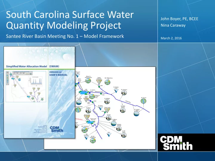
Simplified Water Allocation Model (SWAM)

• Developed in response to an increasing need for a desktop

tool to facilitate regional and statewide water allocation analysis

• Calculates physically and

legally available water, diversions, storage consumption and return flows at user-defined nodes

• Used to support large-scale

planning studies in Colorado, Oklahoma, Arkansas and Texas

The Simplified Water Allocation Model is…

• a water accounting tool
• a WHAT-IF simulation model
• a network flow model that traces water through a natural

stream network, simulating withdrawals, discharges, storage, and hydroelectric operations

• not precipitation-runoff model (e.g., HEC-HMS)
• not a hydraulic model (e.g. HEC-RAS)
• not a water quality model (e.g., QUAL2K)
• not an optimization model
• not a groundwater flow model (e.g., MODFLOW)

The Models Can Be Used To…

• Determine surface-water availability
• Predict where and when future water shortages would occur
• Test alternative water management strategies, new operating

rules, and “what-if” scenarios

• Consolidate hydrologic data
• Evaluate the impacts of future withdrawals on instream flow

needs

• Evaluate interbasin transfers
• Support development of Drought Management Plans
• Compare managed flows to natural flows

River Basin Flow and Operations Models

Similarities between SWAM, OASIS, CHEOPS, and RiverWare:

 Used in major river basin studies and/or statewide water plans  Operating Rules of varying complexity  Monthly and Daily Timesteps  Visual Depiction of the River Network

SWAM

 Familiar and adaptable

environment: Visual Basic and Spreadsheets

 Built in functions for

reservoirs, river

• perations, discharges,

irrigation, return flows, etc.

OASIS

 Built in Probability

Analysis for Real- Time Ops

 Optimization

toward objectives in each timestep

RiverWare

 Fully linked

graphical network development

 3 modes:

 Pure simulation  Rules-based

simulation

 Optimization

Unique Features:

CHEOPS

 Tailored specifically

for hydropower

 Energy

Calculations

 Reservoir

Tracking

 Familiar Visual

Basic programming

Simplified Water Allocation Model (SWAM)

• Object-oriented tool in which a river basin and all of its

influences can be linked into a network with user defined priorities

• Resides within Microsoft Excel
• Point and click setup and
• utput access

Water User Objects

Input Forms Objects Tributaries Discharges Reservoirs Municipal Industrial Golf Courses Power Plants Agriculture Instream Flow Recreational Pool Aquifer USGS Gage Interbasin Transfer

Simplified Water Allocation Model (SWAM)

• Intuitive &

Resides within and interfaces directly with Transparent Microsoft Excel

• Ease-of-Use

Point-and-click setup and output access

• Simple &

Mass balance calculations, but handles Robust

• perating rules, use priorities, etc.

Node Output Input Forms

Simplified Water Allocation Model (SWAM)

• Supports multiple layers of complexity for development of a

range of systems, for example… A Reservoir Object can include:

• 1. Basic hydrology dependent calculations
• 2. Operational rules of varying complexity such as prescribed

releases, conditional releases, or hydrology dependent releases.

Reservoir

SWAM Model Main Screen

MODELING DATA REQUIREMENTS

Santee River Basin

Data Collected for Model Development

• USGS daily flow records
• Historical daily rainfall and evaporation rates
• Historical Operational Data

– Withdrawals (municipal, industrial, agricultural, golf courses) – Discharges – Reservoir elevation

• Reservoir bathymetry and operating rules
• Subbasin characteristics (GIS)

– Drainage area – Land use – Basin slope

• Other data, studies, and models

UNIMPAIRED FLOWS (UIF)

Santee River Basin

UIF Definition and Uses

• Definition: Estimate of natural historic streamflow in the

absence of human intervention in the river channel:

– Storage – Withdrawals – Discharges and Return Flow

• Unimpaired Flow =

Measured Gage Flow + River Withdrawals + Reservoir Withdrawals – Discharge to Reservoirs – Return Flow + Reservoir Surface Evaporation – Reservoir Surface Precipitation + Upstream change in Reservoir Storage + Runoff from Previously Unsubmerged Area

• Fundamental input to the model at headwater nodes and

tributary nodes

• Comparative basis for model results

Primary UIF Data Sources

Documented

• USGS Gage flows
• DHEC records of M&I withdrawals and discharges
• Reservoir operator records of water levels
• Reported agricultural withdrawals
• GIS Data layers

Estimated

• Direct contact with users regarding historic use patterns
• Operational hindcasting
• Agricultural water use modeling

Basinwide UIF Calculation Process

Four Steps in UIF Calculation Process

• Step 1: UIFs for USGS Gages

for individual periods of record

– Involves extension of

• perational data
• Step 2: Extension of UIFs

for USGS Gages through the LONGEST period of record

• Step 3: Correlation

between ungaged basins and gaged basins

• Step 4: UIFs for ungaged

basins

How UIFs are Used in SWAM

Input as upstream tributary flow Calibration/ Validation

• f cumulative

upstream flow

OVERVIEW OF MODEL FRAMEWORK

Santee River Basin

Santee Basin Model Tributaries

Reservoirs and Hydroelectric

21

M&I and Energy Surface Water Withdrawals

Surface Water Withdrawals for Irrigation

Discharges to Surface Water

Interbasin Transfers

Santee Basin – SWAM Framework

Hydropower

MODEL SETUP

Santee River Basin

Two Versions of Every Model

Calibration with UIFs and Historic Use Records Planning with UIFs, Current Uses, and User-Defined Future Uses

Tributary Input Form

Reservoir Input Form

Water User Input Form – Main

Agricultural Water User Input Forms

Instream Flow Input Form

MODEL VALIDATION

Santee River Basin

SWAM Calibration/Validation

• Calibration targets = downstream flow gage records
• Calibration parameters =

– reach gains/losses, – ungaged flow records, – reservoir operations – ag return flow percentages, locations, lags

• Performance metrics =

– Annual avg flows (overall water balance) – Monthly avg flows (seasonality) – Flow percentile distributions (variability, extreme events) – Flow timeseries (specific timings, operations) – Reservoir storage timeseries – CWWMG Inflow Dataset

Calibration Result Graphs

500 1,000 1,500 2,000 2,500 3,000 Aug-87 May-90 Jan-93 Oct-95 Jul-98 Apr-01 Jan-04 Oct-06 Jul-09 Apr-12 Dec-14 SLD09 Saluda nr Ware Shoals (CFS) gaged modeled 200 400 600 800 1,000 1,200 1,400 1,600 Jan Feb Mar Apr May Jun Jul Aug Sep Oct Nov Dec SLD 09 Saluda River nr Ware Shoals Monthly Mean Flow (CFS) gaged modeled 500 1000 1500 2000 2500 3000 0.1 0.2 0.3 0.4 0.5 0.6 0.7 0.8 0.9 1 Precentile SLD09 Saluda River nr Ware Shoals Monthly Flow Percentiles (CFS) gaged modeled

Preliminary examples from the Saluda Basin

THANK YOU

Santee River Basin