
SLIDE 1
12/6/2017 1
SORTING
Chapter 8
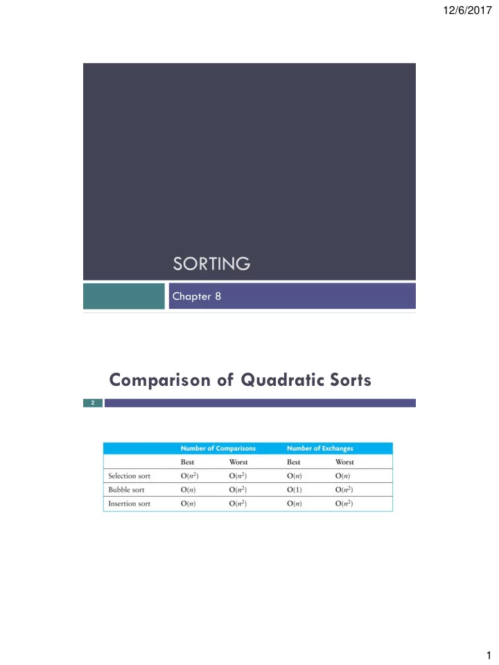
Comparison of Quadratic Sorts
2
SORTING Chapter 8 Comparison of Quadratic Sorts 2 1 12/6/2017 - - PDF document
12/6/2017 SORTING Chapter 8 Comparison of Quadratic Sorts 2 1 12/6/2017 Merge Sort Section 8.7 Merge A merge is a common data processing operation performed on two ordered sequences of data. The result is a third ordered sequence
2
A merge is a common data processing operation
Merge Algorithm
3.
Compare the current items from the two sequences, copy the smaller current item to the output sequence, and access the next item from the input sequence whose item was copied.
For two input sequences each containing n elements,
Merge time is O(n) Space requirements The array cannot be merged in place Additional space usage is O(n)
private static void merge(T[] out, T[] left, T[] right) { // merge left and right into out // Access first item from all sequences int i = 0; // left int j = 0; // right int k = 0; // out // while there is data in both left and right while (i < left.length && j < right.length) { // find smaller and insert into out if (left[i].compareTo(right[j]) < 0)
else
} // Copy remaining items from left into out while (i < left.length)
// Copy remaining items from right into out while (j < right.length)
} // merge()
We can modify merging to sort a single, unsorted
1.
2.
3.
4.
This algorithm can be written with a recursive step
50 60 45 30 90 20 80 15 50 60 45 30 90 20 85 15 30 45 50 60 15 20 80 90 15 20 30 45 50 60 80 90
Each backward step requires a movement of n
The number of steps which require merging is log n
The total effort to reconstruct the sorted array
Requires a total of n additional storage locations.
public static void sort(T[] table) { // A table with 1 element is already sorted if (table.length > 1) { // Split table into halves int halfSize = table.length/2; T[] left = new Comparable[halfSize]; T[] right = new Comparable[table.length – halfSize]; System.arrayCopy(table, 0, left, 0, halfSize); System.arrayCopy(table, halfSize, right, 0, table.length-halfSize); // sort the halves sort(left); sort(right); // merge the halves merge(table, left, right); } } // sort()
Merge sort time is O(n log n) but still requires,
Heapsort does not require any additional storage As its name implies, heapsort uses a heap to store
When used as a priority queue, a heap maintains a smallest value at
The following algorithm places an array's data into a heap, then removes each heap item (O(n log n)) and moves it back into the
array
This version of the algorithm requires n extra storage locations
Heapsort Algorithm: First Version
4.
Remove an item from the queue and insert it back into the array at position i
5.
Increment i
Instead of using a Min Heap, use a Max heap The root contains the largest element Then, move the root item to the bottom of the heap reheap, ignoring the item moved to the bottom
89 76 74 37 32 39 66 20 26 18 28 29 6
6 18 20 26 28 29 32 37 39 66 74 76 89
If we implement
each element
the heap part of
Algorithm for In-Place Heapsort
3.
Remove the first item from the heap by swapping it with the last item in the heap and restoring the heap property
Start with an array table of length
Consider the first item to be a heap of one item Next, consider the general case where the items in
Refinement of Step 1 for In-Place Heapsort
1.1
while n is less than table.length
1.2
Increment n by 1. This inserts a new item into the heap
1.3
Restore the heap property
Because a heap is a complete binary tree, it has log
Building a heap of size n requires finding the
Each insert (or remove) is O(log n) With n items, building a heap is O(n log n) No extra storage is needed
Developed in 1962 Quicksort selects a specific value called a pivot and
all the elements in the left subarray are less than or
all the elements in the right subarray are larger than
The pivot is placed between the two subarrays The process is repeated until the array is sorted
44 75 23 43 55 12 64 77 33
44 75 23 43 55 12 64 77 33 Arbitrarily select the first element as the pivot
55 75 23 43 44 12 64 77 33 Partition the elements so that all values less than or equal to the pivot are to the left, and all values greater than the pivot are to the right
12 33 23 43 44 55 64 77 75 Partition the elements so that all values less than or equal to the pivot are to the left, and all values greater than the pivot are to the right
12 33 23 43 44 55 64 77 75 44 is now in its correct position
12 33 23 43 44 55 64 77 75 Now apply quicksort recursively to the two subarrays
We describe how to do the partitioning later The indexes first and last are the end points of the
The index of the pivot after partitioning is pivIndex Algorithm for Quicksort
2.
Partition the elements in the subarray first . . . last so that the pivot value is in its correct place (subscript pivIndex)
3.
Recursively apply quicksort to the subarray first . . . pivIndex - 1
4.
Recursively apply quicksort to the subarray pivIndex + 1 . . . last
If the pivot value is a random value selected from the
then statistically half of the items in the subarray will be less
If both subarrays have the same number of elements
At each recursion level, the partitioning process involves
Quicksort is O(n log n), just like merge sort
The array split may not be the best case, i.e. 50-50 An exact analysis is difficult (and beyond the scope
A quicksort will give very poor behavior if, each
In that case, the sort will be O(n2) Under these circumstances, the overhead of
We’ll discuss a solution later
public static void sort(T[], int first, int last) { if (first < last) { // partition the table at pivotIndex int pivotIndex = partition(table, first, last); // sort the left half sort(table, first, pivotIndex-1); // sort the right half sort(table, pivotIndex+1, last); } } // sort()
44 75 23 43 55 12 64 77 33
If the array is randomly ordered, it does not matter which element is the pivot. For simplicity we pick the element with subscript first
44 75 23 43 55 12 64 77 33
If the array is randomly ordered, it does not matter which element is the pivot. For simplicity we pick the element with subscript first
Search for the first value at the left end of the array that is greater than the pivot value
up 44 75 23 43 55 12 64 77 33
Then search for the first value at the right end of the array that is less than or equal to the pivot value
up down 44 75 23 43 55 12 64 77 33
Exchange these values
up down 44 75 23 43 55 12 64 77 33
Exchange these values
44 33 23 43 55 12 64 77 75
Repeat
44 33 23 43 55 12 64 77 75
public static void partition(T[] table, int first, int last) { // select first element as pivot value // Initialize up to first and down to last do { // Increment up until it selects first element >= pivot or it reaches last while ((up < last) && (pivot.compareTo(table[up]) >= 0)) up++; // Decrement down until it select first element < pivot or it reaches first while ((down > first) && (pivot.compareTo(table[down]) < 0)) down--; if (up < down) { // exchange table[up] and table[down] T temp = table[up]; table[up] = table[down]; table[down] = temp; } while (up < down); // exchange table[first] and table[down] T temp = table[first]; table[first] = table[down]; table[down] = temp; // return value of down a pivotIndex return down; } // partition()
Quicksort is O(n2) when each split yields one empty
A better solution is to pick the pivot value in a way
Use three references: first, middle, last Select the median of the these items as the pivot
44 75 23 43 55 12 64 77 33
44 75 23 43 55 12 64 77 33 middle first last
44 75 23 43 55 12 64 77 33
Sort these values
middle first last
33 75 23 43 44 12 64 77 55
Sort these values
middle first last
33 75 23 43 44 12 64 77 55
Exchange middle with first
middle first last
44 75 23 43 33 12 64 77 55
Exchange middle with first
middle first last
44 75 23 43 33 12 64 77 55
Run the partition algorithm using the first element as the pivot
Algorithm for Revised partition Method
5. Increment up until up selects the first element greater than the pivot value or up has reached last 6. Decrement down until down selects the first element less than or equal to the pivot value or down has reached first 7. if up < down then 8. Exchange table[up] and table[down]