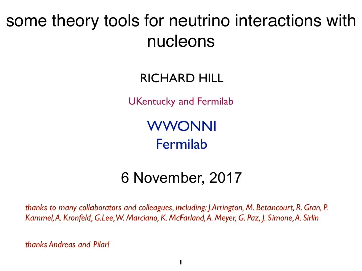
some theory tools for neutrino interactions with nucleons RICHARD - - PowerPoint PPT Presentation

some theory tools for neutrino interactions with nucleons
SMART_READER_LITE
LIVE PREVIEW

some theory tools for neutrino interactions with nucleons RICHARD - - PowerPoint PPT Presentation

some theory tools for neutrino interactions with nucleons RICHARD HILL UKentucky and Fermilab WWONNI Fermilab 6 November, 2017 thanks to many collaborators and colleagues, including: J.Arrington, M. Betancourt, R. Gran, P. Kammel, A.


slide-1
SLIDE 1

some theory tools for neutrino interactions with nucleons

WWONNI Fermilab 6 November, 2017

RICHARD HILL

UKentucky and Fermilab

1

thanks to many collaborators and colleagues, including: J.Arrington, M. Betancourt, R. Gran, P. Kammel, A. Kronfeld, G.Lee,

  • W. Marciano, K. McFarland, A. Meyer, G. Paz, J. Simone, A. Sirlin

thanks Andreas and Pilar!

slide-2
SLIDE 2

2

  • topic 1: amplitude analysis and z expansion
  • topic 2: muon capture and nucleon axial radius

Overview

  • topic 3: radiative corrections and SCET
  • topic 0: why
slide-3
SLIDE 3

3

topic 0. why

slide-4
SLIDE 4

4

why bother with neutrino interactions? Isn’t this too hard/ too different/ somebody else’s problem?

topic 0. why

slide-5
SLIDE 5

4

why bother with neutrino interactions? Isn’t this too hard/ too different/ somebody else’s problem?

topic 0. why

“The good news is that it’s not my problem”

HEP

slide-6
SLIDE 6

10 20 30 200 400 600 800 1000 (GeV)

ν

E 1 10 CC evts/GeV/10kt/MW.yr

µ

ν 200 400 600 800 1000 Appearance Probability 0.02 0.04 0.06 0.08 0.1 0.12 0.14 0.16 0.18 0.2

CC spectrum

µ

ν =n/a

cp

δ = 0.0,

13

θ 2

2

sin /2 π =-

cp

δ = 0.1,

13

θ 2

2

sin =0

cp

δ = 0.1,

13

θ 2

2

sin /2 π =+

cp

δ = 0.1,

13

θ 2

2

sin

2

= 2.4e-03 eV

31 2

m ∆ CC spectrum at 1300 km,

µ

ν

5

long baseline neutrino oscillation experiment is simple in conception:

LBNE, 1307.7335

slide-7
SLIDE 7

10 20 30 200 400 600 800 1000 (GeV)

ν

E 1 10 CC evts/GeV/10kt/MW.yr

µ

ν 200 400 600 800 1000 Appearance Probability 0.02 0.04 0.06 0.08 0.1 0.12 0.14 0.16 0.18 0.2

CC spectrum

µ

ν =n/a

cp

δ = 0.0,

13

θ 2

2

sin /2 π =-

cp

δ = 0.1,

13

θ 2

2

sin =0

cp

δ = 0.1,

13

θ 2

2

sin /2 π =+

cp

δ = 0.1,

13

θ 2

2

sin

2

= 2.4e-03 eV

31 2

m ∆ CC spectrum at 1300 km,

µ

ν

5

long baseline neutrino oscillation experiment is simple in conception:

Measure fraction

  • f νe appearing

in νμ beam

LBNE, 1307.7335

slide-8
SLIDE 8

10 20 30 200 400 600 800 1000 (GeV)

ν

E 1 10 CC evts/GeV/10kt/MW.yr

µ

ν 200 400 600 800 1000 Appearance Probability 0.02 0.04 0.06 0.08 0.1 0.12 0.14 0.16 0.18 0.2

CC spectrum

µ

ν =n/a

cp

δ = 0.0,

13

θ 2

2

sin /2 π =-

cp

δ = 0.1,

13

θ 2

2

sin =0

cp

δ = 0.1,

13

θ 2

2

sin /2 π =+

cp

δ = 0.1,

13

θ 2

2

sin

2

= 2.4e-03 eV

31 2

m ∆ CC spectrum at 1300 km,

µ

ν

5

long baseline neutrino oscillation experiment is simple in conception:

Measure fraction

  • f νe appearing

in νμ beam Do it as a function

  • f energy

LBNE, 1307.7335

slide-9
SLIDE 9

6

long baseline neutrino oscillation experiment is difficult in practice: simple picture is complicated by

  • intrinsic νe component of beam
  • degeneracy of uncertainty in detector response and

neutrino interaction cross sections

  • imperfect energy reconstruction
  • νe versus νμ cross section differences

need theory for σνe/σνμ, at ~% precision of measurement and also

  • beam divergence and oscillation (near flux≠far flux)

aided by near detector but need theory for σνμ, at a precision depending on the experimental capabilities

slide-10
SLIDE 10

7

current paradigm: constrain neutrino interactions by

  • determining nucleon level amplitudes
  • parameterizing/measuring/calculating nuclear

modifications folk paradigms: constrain neutrino interactions by

  • starting at the quark level
  • computing nuclear response

constrain neutrino interactions by

  • starting directly at the nuclear level
  • parameterizing and measuring every cross section

“perfect theory” “perfect expt.”

slide-11
SLIDE 11

8

in any paradigm: near detector has access to primarily νμ neutrinos νe appearance signal is directly impacted by νμ/νe cross section differences

  • kinematics
  • 2nd class currents (G parity violation)
  • radiative corrections (QED and EW)
  • signal definition

having talked the talk, do some walking:

  • νμ/νe in the time reversal process (μ p → ν n)
  • nucleon input uncertainty (e-p, ν d → ν n)
  • radiative corrections at GeV (e-p)

nuclear corrections: see talks of W. Van Order, S. Pastore, A. Ankowski, N. Jachowicz, A. Lovato. experiment: S. Bolognesi; lots of references: NUSTEC white paper 1706.03621

slide-12
SLIDE 12

9

beyond neutrino oscillations related applications relying on quantitative nucleon structure:

  • fundamental constants (probable 7 sigma shift in Rydberg)
  • sigma terms and WIMP-DM direct detection
  • gA and BBN

entering a precision realm where percent level corrections to nucleon structure need to be calculated, not just estimated QED is “easy”. But QED + nucleon structure is “hard” Notes:

slide-13
SLIDE 13

10

topic 1. amplitude analysis and z expansion

first, e-p elastic scattering second, ν-n CC scattering

slide-14
SLIDE 14

11

topic 1. amplitude analysis and z expansion

first, e-p elastic scattering second, ν-n CC scattering

slide-15
SLIDE 15

recall scattering from extended classical charge distribution:

e−

e− ρ(r)

dσ dΩ = ✓ dσ dΩ ◆

pointlike

|F(q2)|2

for the relativistic, QM, case, define radius as slope of form factor

F(q2) = Z d3r eiq·rρ(r) = Z d3r  1 + iq · r 1 2(q · r)2 + . . .

  • ρ(r)

= 1 1 6hr2iq2 + . . .

hJµi = γµF1 + i 2mp σµνqνF2

GE = F1 + q2 4m2

p

F2

GM = F1 + F2

r2

E ≡ 6 d

dq2 GE(q2)

  • q2=0

12

(up to radiative corrections)

slide-16
SLIDE 16

Radius extraction requires data over a Q2 range where a simple Taylor expansion of the form factor is invalid

maximum Q2 [GeV2] radius error [fm]

[sensitivity studies based on bounded z expansion fit]

13

data of Bernauer et al. (A1 collaboration), PRL 105, 242001 (2010)

slide-17
SLIDE 17

Radius extraction requires data over a Q2 range where a simple Taylor expansion of the form factor is invalid

maximum Q2 [GeV2] radius error [fm]

size of rE anomaly (hydrogen) [sensitivity studies based on bounded z expansion fit]

13

data of Bernauer et al. (A1 collaboration), PRL 105, 242001 (2010)

slide-18
SLIDE 18

Radius extraction requires data over a Q2 range where a simple Taylor expansion of the form factor is invalid

maximum Q2 [GeV2] radius error [fm]

size of rE anomaly (hydrogen) [sensitivity studies based on bounded z expansion fit]

13

Cut used for radius extraction

data of Bernauer et al. (A1 collaboration), PRL 105, 242001 (2010)

slide-19
SLIDE 19

Radius extraction requires data over a Q2 range where a simple Taylor expansion of the form factor is invalid

maximum Q2 [GeV2] radius error [fm]

size of rE anomaly (hydrogen) convergence radius for simple Taylor expansion [sensitivity studies based on bounded z expansion fit]

13

Cut used for radius extraction

data of Bernauer et al. (A1 collaboration), PRL 105, 242001 (2010)

slide-20
SLIDE 20

14

coefficients in rapidly convergent expansion encode nonperturbative QCD

tcut F(q2) = X

k

ak[z(q2)]k

experimental kinematic region That’s ok: underlying QCD tells us that Taylor expansion

  • f form factor in appropriate variable is convergent

q2

particle thresholds

z

z(q2, tcut, t0) = p tcut − q2 − √tcut − t0 p tcut − q2 + √tcut − t0 ,

slide-21
SLIDE 21

15

Reanalysis of scattering data reveals strong influence of shape assumptions Errors larger, but discrepancy remains

proton radius[fm]

electron combination

2S − 2P 1

2

2S − 2P 1

2

2S − 2P 3

2

2S − 4S 1

2

2S − 4D 5

2

2S − 4P 1

2

2S − 4P 3

2

2S − 6S 1

2

2S − 6D 5

2

2S − 8S 1

2

2S − 8D 3

2

2S − 8D 5

2

2S − 12D 3

2

2S − 12D 5

2

1S − 3S 1

2

Mainz data

  • ther world data

muonic H

slide-22
SLIDE 22

15

Reanalysis of scattering data reveals strong influence of shape assumptions Errors larger, but discrepancy remains

proton radius[fm]

electron combination

2S − 2P 1

2

2S − 2P 1

2

2S − 2P 3

2

2S − 4S 1

2

2S − 4D 5

2

2S − 4P 1

2

2S − 4P 3

2

2S − 6S 1

2

2S − 6D 5

2

2S − 8S 1

2

2S − 8D 3

2

2S − 8D 5

2

2S − 12D 3

2

2S − 12D 5

2

1S − 3S 1

2

Mainz data

  • ther world data

reanalysis of Mainz data reanalysis of other world data Lee, Arrington, Hill (2015)

muonic H

slide-23
SLIDE 23

16

0.8 0.9 1 1.1

2S − 2P1/2 2S − 2P1/2 2S − 2P3/2 2S − 4S 1/2 2S − 4D5/2 2S − 4P1/2 2S − 4P3/2 2S − 6S 1/2 2S − 6D5/2 2S − 8S 1/2 2S − 8D3/2 2S − 8D5/2 2S − 12D3/2 2S − 12D5/2 1S − 3S 1/2

e-p Mainz e-p world CODATA 2010 electron comb. e-p Mainz (z exp.) e-p world (z exp.) CODATA 2014 electron comb. µD + iso. H 2S-4P (sensitivity) low-Q2 e-p (sensitivity) µ-p (sensitivity)

rp

E (fm)

CREMA µH 2010→ CREMA µH 2014→

update: Beyer et al. (Science, 2017)

slide-24
SLIDE 24

17

topic 1. amplitude analysis and z expansion

first, e-p elastic scattering second, ν-n CC scattering

slide-25
SLIDE 25

18

Start with the basic process

n p μ- νμ

poorly known axial-vector form factor

σ(νn → µp) = | · · · FA(q2) · · · |2

A common ansatz for FA has been employed for the last ~40 years:

F dipole

A

(q2) = FA(0) ✓ 1 − q2 m2

A

◆2

rA = 0.674(9) fm

1 FA(0) dFA dq2

  • q2=0

⌘ 1 6r2

A

Typically quoted uncertainties are (too) small (e.g. compared to proton charge form factor!) Inconsistent with QCD.

slide-26
SLIDE 26

19

n p μ- νμ p p

deuteron Deuterium bubble chamber data

Fermilab 15-foot deuterium bubble chamber, PRD 28, 436 (1983)

  • small statistics, ~3000 events in world data
  • small(-ish) nuclear effects
  • small(-ish) experimental uncertainties

28

HIGH-ENERGY QUASIELASTIC v„n ~@ p SCATTERING IN. . . 439

80

60

Ot

P co.

h4, =1.05 GeV

tion, the

following assumptions

are made:

(1) time-

reversal invariance and charge symmetry, (2) partially

con-

served axial-vector

current

(PCAC} for the small pseudo-

scalar term,

and

(3) isotriplet-conserved-vector-current

(CVC) hypothesis. The first assumption,

which requires all form factors to

be real, yields Eq —

F~—

0, leading to the absence of second

class currents. With the second

assumption,

Fp(Q

) is

given by

20-

Fp(Q )=2M Fg(Q~)/(Q

+m ),

where

'0

2

Q' (Gev')

  • FICx. S.

The

Q distribution

for the

selected quasielastic events.

The solid curve represents

the differential

cross section

  • f quasielastic

scattering for the neutron

in deuteron.

Q'= (P —

P„)'—

(E„—

E„)' .

The contribution to the cross section from this term in the

energy region E„&5 GeV is less than 0.1%, and conse- quently

this term is neglected.

The third

assumption re- lates Fz and Fz to the isovector Sachs electric and mag- netic form factor, Gz and G~ determined from electron- scattering experiments as follows: near /=0 . The shaded area corresponds

to the addition-

al events found from the rescan. Using the average of the events with P between —

90

and

126

(dashed line), we calculated

the event bias to be

S%%uo. This does not neces-

sarily represent

the true

loss of events because

  • f the

three-point plot per event.

We examined the true event

loss from the event bias in Fig. 4 by using a Monte Carlo simulation.

This

event loss amounts

to 8% and

is not recovered by rescanning (shaded

area).

Hence, a correc- tion of 1.08+0.05 has been made to the data independent

  • f scanning

efficiency. Figure

5 shows

the Q distribution

for the quasielastic

events.

The curve in Fig. 5 is the best fit obtained

by us- ing the prediction of the differential

cross section for reac- tion

(2) with

M~ —

1.05 GeV which

was obtained

from this experiment

(see Sec. III). The X value from this ftt was found to be 15 for 20 data points for Q between 0.1 and 3 GeV . Comparing

the observed Q distribution

to

the fitted curve, the correction factor for Q &0.1 GeV2 is estimated

to be 1.10+0.02. The overall

correction factor

including scanning-measuring

efficiency

is

1.34+0.07.

We note that this correction factor influences the value of

the neutrino flux but not the Mz value, because we use a flux-independent method

to determine

Mq.

  • III. MEASUREMENT OF THE FORM FACTOR

2 2

Fy(Q') = G~(Q')+

G (Q')

1+

4M 4M

2

' — 1

Ff(Q )=[6M(Q

)—

GE(Q )]g

' 1+ 4M

2

' —

2

GE(Q }=6M(Q }(1+/)

=A(Q

) 1+

My

where M~ is the vector mass, Mv —

0.84 GeV, g is the

difference

between

the proton

and neutron anomalous magnetic moment,

g'=}Mp —

p„=3.708,

and

A,(Q

) (Ref. 1S) is the correction factor for the small

deviation

  • f the electron-scattering

data from a pure di-

pole

form

factor.

We further

assume

the axial-vector form factor in a dipole form,

+g(Q )=+g(0)/(I+Q

/Mg

)

where

the value of F~(0)= —

1.23+0.01 is taken from P-

decay experiments. '

From these

assumptions, the differential

cross section

for the quasielastic

reaction can be expressed

in terms of

  • nly one parameter,

Mz, as

In the context of the V—

A theory,

the matrix

element

for the quasielastic

reaction,

v&n ~p p, can be written

as

a product of the hadronic

weak current and the leptonic

  • current. '

The general

form of the hadronic

weak current is written in terms of six complex form factors which are

functions

  • f Q

and

characterize

the nucleon

structure. These are Fs (induced scalar), Fp (induced pseudoscalar),

F~ (isovector

Dirac), Ff (isovector

Pauli), F~ (axial vec-

tor}, and Fr (induced

tensor).

The quasielastic

cross sec- tion can be expressed

in terms of these six form factors.

In order to simplify

the analysis of the quasielastic reac-

GMcos8c

2

2 (s

u)

&( ')+&(

)

dQ

8rrE„M

1

C(Q2) (s —

u)

(7)

where

s —

u =4ME„Q

m&,

and M =(M„+—

Mp)—

/2.

The values of the Fermi constant

and of the Cabibbo angle

are taken

to

be G = 1.166 32 & 10

GeV

and

cos8c —

0.9737, respectively

(see Ref. 16). The structure

Best source of almost-free neutrons: deuterium

ANL 12-foot deuterium bubble chamber, PRD 26, 537 (1982) BNL 7-foot deuterium bubble chamber, PRD23, 2499 (1981) also:

slide-27
SLIDE 27

20

[a1, a2, a3, a4] = [2.30(13), −0.6(1.0), −3.8(2.5), 2.3(2.7)] (31)

Cij = B B B @ 1 0.350 −0.678 0.611 0.350 1 −0.898 0.367 −0.678 −0.898 1 −0.685 0.611 0.367 −0.685 1 1 C C C A

  • FA with complete error budget:

]

2

[GeV

2

Q

1 2 3

)

2

(-Q

A

F

0.5 1

=4 z expansion

a

N = 1.014(14) dipole

A

m

z

  • 0.2

0.2 0.4

(z)

A

F

0.5 1

=4 z expansion

a

N = 1.014(14) dipole

A

m

slide-28
SLIDE 28

21

Derived observables: 1) axial radius

1 FA(0) dFA dq2

  • q2=0

⌘ 1 6r2

A

  • order of magnitude larger uncertainty compared to historical dipole fits
  • impacts comparison to other data, e.g. pion electroproduction, muon

capture

r2

A = 0.46(22) fm2 .

slide-29
SLIDE 29

22

Derived observables: 2) neutrino-nucleon quasi elastic cross sections

[GeV]

ν

E

  • 1

10 1 10

]

2

)[cm

ν

(E σ

5 10 15

  • 39

10 ×

=4 z expansion

a

N = 1.014(14) dipole

A

m

[GeV]

ν

E

  • 1

10 1 10

]

2

)[cm

ν

(E σ

5 10 15

  • 39

10 ×

=4 z expansion

a

N = 1.014(14) dipole

A

m

σνn→µp(Eν = 1 GeV) = 10.1(0.9) × 10−39 cm2

−39 2

× σνn→µp(Eν = 3 GeV) = 9.6(0.9) × 10−39 cm2

slide-30
SLIDE 30

]

2

[GeV

2

Q

0.5 1 1.5 2

]

2

/GeV

2

[cm

2

/dQ σ d

5 10 15 20

  • 39

10 ×

GENIE RFG z-expansion GENIE RFG dipole MINERvA Data

23

discriminating nuclear models

n p μ- νμ poorly known axial form factor

σ(νn → µp) = | · · · FA(q2) · · · |2

want to extract nuclear and flux effects from this comparison: but large nucleon level form factor uncertainty

slide-31
SLIDE 31

24

topic 2. muon capture

slide-32
SLIDE 32

25

W + p µ− n νµ

muon capture from ground state of muonic hydrogen:

  • probes axial nucleon structure: FP

, FA

  • already competitive determination of rA
  • potential for significant improvement

from RJH, Kammel, Marciano, Sirlin 1708.08462

slide-33
SLIDE 33

26

W + p µ− n νµ

L = GF Vud p 2 ¯ νµγµ(1 γ5)µ ¯ dγµ(1 γ5)u + H.c. + . . . ,

H = p2 2mr α r + δVVP iG2

F |Vud|2

2 ⇥ c0 + c1(sµ + sp)2⇤ δ3(r) ,

Λ = G2

F |Vud|2 ⇥ [c0 + c1F(F + 1)] ⇥ |ψ1S(0)|2 + . . .

perturbative matching nonperturbative matching

L = LSM

weak hadronic atomic

}

factorization:

}

}

c0 = E2

ν

2πM2 (M mn)2 2M mn M mn F1(q2

0) + 2M + mn

M mn FA(q2

0) mµ

2mN FP (q2

0)

+ (2M + 2mn 3mµ)F2(q2

0)

4mN 2 , ⇢

slide-34
SLIDE 34

27

W + γ p µ− n νµ

expansion in small quantities:

✏ ∼ ↵ ∼ m2

µ

m2

ρ

∼ mu − md mρ . 10−2

  • axial radius enters at first order in epsilon, so need all other first
  • rder corrections (to ~10%, for a 10% measurement of rA2)
  • will see that other corrections are at first-and-a-half order; need to

ensure against numerical enhancements (need these to ~100%)

slide-35
SLIDE 35

28

momentum expansion:

q2

0 ⌘ m2 µ 2mµEν = 0.8768 m2 µ.

1 +  g1, gA

  • + √✏

 g2

  • + ✏

 r2

1, r2 A, gP

  • + . . .

sensitivity to momentum dependence in the capture process in our power counting, rA2 competes with gP , and other well-determined quantities (g≡normalization, r2≡slope)

∼ ✏

FP (q2

0) = 2mNgπNNfπ

m2

π − q2

− 1 3 gA m2

N r2 A + . . .

gpiNN: pion-nucleon scattering, and NN scattering

gA: neutron lifetime

g1,g2,r12: e-p, e-n scattering + H, muH (see below)

✔ ✔

slide-36
SLIDE 36

29

α expansion: Sirlin g function (IR subtraction)

RC = RC(electroweak) + RC(finite size) + RC(electron VP) ,

matching, running in 4 Fermi theory

}

hadronic matrix element

}

computed within QM

}

RC(electroweak) = α 2π  4 log mZ mp 0.595 + 2C + g(mµ, βµ = 0)

  • + · · · = +0.0237(10) ,

RC(electron VP) = +0.0040(2),

RC(finite size) = 0.005(1)

} }

finite terms (estimate with OPE) large log

}

(should be done better: computed in large nucleus ansatz rE>>rA)

✔ ✔ ✔

slide-37
SLIDE 37

30

isospin violation:

hn|(V µ Aµ)|pi = ¯ un  F1(q2)γµ+ iF2(q2) 2mN σµνqν FA(q2)γµγ5 FP (q2) mN qµγ5 + FS(q2) mN qµ iFT (q2) 2mN σµνqνγ5

  • up + . . . ,

vector form factors: CC from isovector NC 2nd class currents: deviations in F1(0): second order in IV (definition of CVC) deviations in F1(q2): first order in IV plus first order in q2 deviations in F2(0): first order in IV plus 0.5 order in kinematic prefactor (numerical estimate: 3.2e-4 << %)

✔ ✔ ✔

contribution of FS,FT: first order in IV plus 0.5 order in kinematic prefactor

slide-38
SLIDE 38

31

results:

¯ gP

MuCap

  • r2

A=0.46(22) fm2 = 8.19 (48)exp (69)¯

gA (6)RC = 8.19(84)

¯ gP

theory = 8.25(25)

gMuCap

πNN

= 13.04 (72)exp (8)gA (67)r2

A (10)RC = 13.04(99)

, gexternal

πNN

= 13.12(10)

r2

A(MuCap) = 0.43 (24)exp (3)gA (3)gπNN (3)RC = 0.43(24) fm2.

turning the tables, take QCD for granted and extract rA2: competitive with other methods with existing data, and potential for improvement

A

δr2

A(future exp.) = (0.08)exp (0.03)gA (0.03)gπNN (0.03)RC = 0.10 fm2.

factor 3 improvement

slide-39
SLIDE 39

32

0.2 0.4 0.6 0.8 1

r2

A (fm2)

νd (dipole) [17] eN → eNπ (dipole) [17] νC (dipole) [20] νd (z exp.) [19] MuCap this work LHPC [21] ETMC [22] CLS [23] PNDME [24] lattice QCD             

W + p µ− n νµ

  • potential factor ~3 improvement from next generation muon capture

experiment

muon capture constraints

lattice average: see also Yao, Alvarez-Ruso, Vicente-Vacas 1708.08776 [ rA2=0.26(4) ] RJH, Kammel, Marciano, Sirlin 1708.08462

complete error budgets

slide-40
SLIDE 40

33

2 4 6 8 10 0.7 0.8 0.9 1 1.1 1.2

Eν (GeV) σ (10−38cm2)

existing error (no external radius constraint) with radius constraint: ( hatched:

external radius error δrA2=20% )

implications for quasielastic neutrino cross sections

slide-41
SLIDE 41

34

0.2 0.4 0.6 1.26 1.27 1.28 1.29

r2

A (fm2)

gA

δΛ = 1% δΛ = 0.33%

test of electron-muon universality

electron coupling (neutron lifetime) current uncertainty muon coupling (current uncertainty)

slide-42
SLIDE 42

35

topic 3. radiative corrections and SCET

slide-43
SLIDE 43

36

  • eikonal coupling
  • factorization of soft region

p p p p p p p p

p p p p

k µ p

p p

( (

= e pµ p · k

  • proof by induction

⇒ exponentiation of IR divergences, cancellation between real and virtual

+ . . .

Yennie, Frautschi, Suura (1961)

But exponentiation of IR divergences does not imply exponentiation of the entire first order correction

slide-44
SLIDE 44

Large logarithms spoil QED perturbation theory when -q2=Q2~GeV2

+

|F(q2)|2 → |F(q2)|2 ✓ 1 − α π log Q2 m2

e

log E2 (∆E)2 + . . . ◆

}

≈ 0.5

Experimental ansatz sums exponentiates 1st order:

|F(q2)|2 ✓ 1 − α π log Q2 m2

e

log E2 (∆E)2 + . . . ◆ → |F(q2)|2 exp  − α π log Q2 m2

e

log E2 (∆E)2

  • Captures leading logarithms when

Q ∼ E , ∆E ∼ me

As consistency check, error budget should contain the difference from resumming:

log2 Q2 m2

e

log Q2 m2

e

log E2 (∆E)2

vs.

e− e− e− e−

37

∆E q e− e−

slide-45
SLIDE 45

38

0.75 0.80 0.85 0.90 0.95 1.00 rE [fm] 0.0 0.1 0.2 0.3 0.4 0.5 0.6 0.7 0.8 0.9 1.0 Q2

max [GeV2]

0.6

Q2 [GeV2] δ

1st order in α 2nd order in α

  • quoted systematics in A1 electron-proton

scattering data are 0.2-0.5 %

  • need to systematically account for

subleading logarithms, recoil, nuclear charge and structure

  • leading order radiative corrections ~30%

total radiative correction

∆E = 5 MeV

electron energy loss cut:

E = 1 GeV

electron energy:

slide-46
SLIDE 46

38

0.75 0.80 0.85 0.90 0.95 1.00 rE [fm] 0.0 0.1 0.2 0.3 0.4 0.5 0.6 0.7 0.8 0.9 1.0 Q2

max [GeV2]

0.6

}

> 5σ discrepancy

Q2 [GeV2] δ

1st order in α 2nd order in α

  • quoted systematics in A1 electron-proton

scattering data are 0.2-0.5 %

  • need to systematically account for

subleading logarithms, recoil, nuclear charge and structure

  • leading order radiative corrections ~30%

total radiative correction

∆E = 5 MeV

electron energy loss cut:

E = 1 GeV

electron energy:

slide-47
SLIDE 47

38

0.75 0.80 0.85 0.90 0.95 1.00 rE [fm] 0.0 0.1 0.2 0.3 0.4 0.5 0.6 0.7 0.8 0.9 1.0 Q2

max [GeV2]

0.6

}

potentially large uncertainty from radiative corrections

Q2 [GeV2] δ

1st order in α 2nd order in α

  • quoted systematics in A1 electron-proton

scattering data are 0.2-0.5 %

  • need to systematically account for

subleading logarithms, recoil, nuclear charge and structure

  • leading order radiative corrections ~30%

total radiative correction

∆E = 5 MeV

electron energy loss cut:

E = 1 GeV

electron energy:

slide-48
SLIDE 48

39

p p ⇥ p p ⇥

+ + +

treat the problem in stages:

proton electron

p p ⇥

p p p p

⇥⇥

static source,

  • nonrel. limit

static source,

  • rel. limit

with recoil corrections with nuclear charge corrections (two photon exchange)

slide-49
SLIDE 49

40

dσ / H ✓Q2 µ2 ◆ J ✓m2 µ2 ◆ R ✓m2 µ2 , p · p0 m2 ◆ S ✓∆E µ , p · p0 m2 , E m, E0 m ◆

=

+ +

+

}

}

  • factorization

hadron structure (Born form factors, …) hard collinear soft

[ remainder function starting at 2-loop (collinear anomaly/rapidity logs) ]

  • physical electron mass regulates collinear divergences
  • R given by ratio of Wilson loop matrix elements in m≠0/m=0

Becher, Melnikov (2007) Chiu, Golf, Kelley, Manohar (2007) Becher, Neubert (2010) Chiu, Jain, Neill, Rothstein (2012) …

slide-50
SLIDE 50

41

Hard

Large logarithms regardless of choice for μ FS: exponentiates (evaluate at any scale) FJ: evaluate at μ~m FH: evaluate at μ~M~Q

FH(µ) = 1 + α 4π  − log2 Q2 µ2 + 3 log Q2 µ2 − 8 + π2 6

  • Soft

FS(µ) = 1 + α 4π  2 log λ2 µ2 ✓ log Q2 m2 − 1 ◆

Collinear FJ(µ) = 1 + α

4π  log2 m2 µ2 − log m2 µ2 + 4 + π2 6

  • F = FHFJFS

Sudakov form factor at one loop: (two-loop matching, real+virtual see 1605.02613)

slide-51
SLIDE 51

42

Two photon exchange

  • Nuclear charge corrections introduce new spin structures

(helicity counting: 3 amplitudes at leading power in me/Q)

FH(µ)γµ ⊗ γµ →

3

X

i=1

ci(µ) Γ(e)

i

⊗ Γ(p)

i

  • In principle, can use e+ and e- data to separately determine

1-photon exchange and 2-photon exchange contributions to ci

  • However, with available data, measure combination of 1-

photon and 2-photon contributions.

  • Regardless of treatment of hard coefficients, remaining

radiative corrections are universal

slide-52
SLIDE 52

43

p S(µ, ∆E = 0) = Z(e)

h Z(p) h

  • +

+ + + + +

  • ⇢⇥

⇤ ⇥ ⇤

want to extract this

}

correct data by this factor

  • J: refers to collinear region, same as before
  • S: include nuclear charge for general soft function (computed through 2-

loop order)

  • H(μ)/H(M): must now account for large logs in this factor

dσ = H(M) × H(µ) H(M) × J(µ) × S(µ)

slide-53
SLIDE 53

44

  • resummation

d log H d log µ = 2  γcusp(¯ α) log Q2 µ2 + γcusp(v · v0, ¯ α) + 2γcusp(¯ α) log v · p0 −v · p − i0 + γ(¯ α)

  • .

proton : Mvµ electron : pµ

universal functions

log H(µL) H(µH) = − α 2π log2 µ2

H

µ2

L

+ . . .

¯ hiv · Dh → ¯ h(0)S†

viv · DSvh(0) = ¯

h(0)iv · ∂h(0) , Sv(x) = P exp  i Z 0

−∞

dsv · As(x + sv)

  • v

v0 governed by Wilson loops with cusps: renormalization of hard function of interest: solution, summing large logarithms:

slide-54
SLIDE 54

45

)

2

(GeV

2

Q

0.2 0.4 0.6 0.8 1

δ

0.35 − 0.3 − 0.25 − 0.2 − 0.15 −

total radiative correction

LL NLL NLO

}

dσ = H(M) × H(µ) H(M) × J(µ) × S(µ)

total radiative correction

numerically: αL2 = α log2 Q2

m2 ∼ 1

αL ∼ α

1 2

, etc.

O(1) O(α

1 2 )

O(α)

correct through:

∆E = 5 MeV

electron energy loss cut:

E = 1 GeV

electron energy:

slide-55
SLIDE 55

46

Comparison to previous implementations of radiative corrections, e.g. in A1 analysis of electron-proton scattering data

)

2

(GeV

2

Q

0.2 0.4 0.6 0.8 1

δ

0.25 − 0.24 − 0.23 − 0.22 − 0.21 − 0.2 −

resummed EFT result naive exponentiation of 1-loop, (μ2=Q2 in two-photon piece) naive exponentiation of 1-loop, (μ2=M2 in two-photon piece)

  • complete analysis: account for floating normalizations, correlated

shape variations when fitting together with backgrounds

  • discrepancies at 0.5-1% compared to currently applied radiative

correction models (cf. 0.2-0.5% systematic error budget of A1 experiment)

  • conflicting implicit scheme choices for 1PE and 2PE

total radiative correction

∆E = 5 MeV E = 1 GeV

slide-56
SLIDE 56

47

EFT analysis clarifies several issues involving conflicting and/or implicit conventions and scheme choices

1) Scheme choice and definition of radius and “Born” form factors 2) Scheme dependence of two-photon exchange 3) Limitations of naive exponentiation

slide-57
SLIDE 57

48

1) Scheme choice and definition of radius and “Born” form factors Fi(q2)Born ⌘ ˜ Fi(q2)F 1

S (w, µ = M)

hJµi = ¯ uv0  ˜ F1γµ + ˜ F2 i 2σµν(v0

ν vν)

  • uv ,

hard coefficient soft function

˜ Fi = FHFS

Multiple conventions in the literature. Different “Born” form factors, different radii (differences typically below current precision)

FH(q2, µ = M) ≡

Massive particle form factor (e.g. for proton):

slide-58
SLIDE 58

49

2) Scheme dependence of two-photon exchange

As for form factors, define hadronic functions in the general 2→2 scattering process as the hard component in the factorization formula at factorization scale μ=M Prevailing conventions have used conflicting μ=M for 1 photon exchange, μ=Q for 2 photon exchange

)

2

(GeV

2

Q

0.2 0.4 0.6 0.8 1

δ

0.25 − 0.24 − 0.23 − 0.22 − 0.21 − 0.2 −

A scale-variation estimate of uncertainty in the 2 photon exchange subtraction μ=M μ=Q

total radiative correction

slide-59
SLIDE 59

50

3) Limitations of naive exponentiation

⇒ New terms at order α2 L3, α2 L2, α3 L4, …

S(2) = 1 2![S(1)]2 − 16π2 3 (L − 1)2 .

⇒ New terms at order α2 L2

  • Total versus individual real photon energy below ΔE :

log H(µL) H(µH) = − α 2π log2 µ2

H

µ2

L

+ . . .

  • Renormalization analysis for subleading logs :

complete analysis: account for floating normalizations, correlated shape variations when fitting together with backgrounds.

S = X

n

⇣ α 4π ⌘n S(n)

a difficult archeological problem. PRP from e-p appears to require something more (expt. syst.: ? / theory systematic: hard TPE)

slide-60
SLIDE 60

51

summary

slide-61
SLIDE 61

52

  • topic 1: amplitude analysis and z expansion: need to do

better for elementary amplitudes

  • topic 2: muon capture: template for general νe/νμ analysis

and world’s best (in a tie) rA determination

Summary

  • topic 3: radiative corrections and SCET: template for

exclusive νe/νμ analysis and cautionary tale for % level

  • topic 0: critical theory input needed for νe/νμ cross section

differences and ν amplitudes at the nucleon level