
SLIDE 1
Hopfield Network
- !
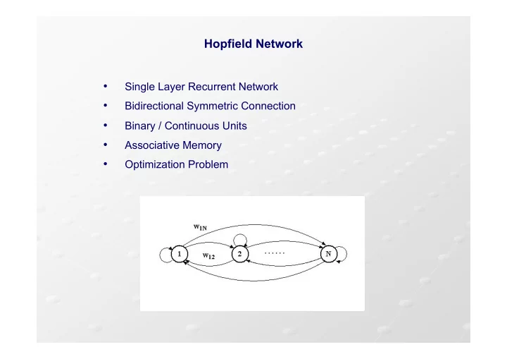
Single Layer Recurrent Network
- !
Bidirectional Symmetric Connection
- !
Binary / Continuous Units
- !
Associative Memory
- !
Optimization Problem