[PPT] - Simulations of the quadrilateral- -based based Simulations of the PowerPoint Presentation

SLIDE 1

9/15/05 Jie Gao CSE590-fall05 1

Simulations of the quadrilateral Simulations of the quadrilateral-

based

based localization localization

Cluster success rate v.s. node degree.
Each plot represents a simulation run.

SLIDE 2

9/15/05 Jie Gao CSE590-fall05 2

Random deployment Random deployment

Poisson distribution does not look uniform.
~400 nodes, average degree is about 5.

SLIDE 3

9/15/05 Jie Gao CSE590-fall05 3

Random deployment Random deployment

Poisson distribution does not look uniform.
~800 nodes, average degree is about 10.

SLIDE 4

9/15/05 Jie Gao CSE590-fall05 4

What you can do & what you can not do What you can do & what you can not do by using angles by using angles… …

SLIDE 5

9/15/05 Jie Gao CSE590-fall05 5

Localization by distance information Localization by distance information

Flipping causes the trouble, especially for sparse

graph.

Intuition: angle information helps to eliminate

incorrect flips.

SLIDE 6

9/15/05 Jie Gao CSE590-fall05 6

Lemma: By local angles of a unit-disk graph, we can determine all pairs of crossing edges in a valid embedding.

What does angle information buy us? What does angle information buy us?

If AB crosses CD in UDG, then by the crossing lemma, one of them, say B, has edges to the other three nodes.

SLIDE 7

9/15/05 Jie Gao CSE590-fall05 7

Local angle information Local angle information

Using local angle information only can not solve the

localization problem in the worst case – UDG embedding is NP-hard with only local angle info.

Preliminary experiments show the effectiveness of

using angle information in sparse graphs.

More to be explored as to what one can do with angle

information.

SLIDE 8

9/15/05 Jie Gao CSE590-fall05 8

Local angle info Local angle info UDG embedding UDG embedding

NP NP-

hard

hard

SLIDE 9

9/15/05 Jie Gao CSE590-fall05 9

l l

6 11

l

3 2

l

3 2

l

3 2

l

3 2 Consider a unit-disk graph, where the two ‘teeth’ do not cross:

Yet a different ambiguity Yet a different ambiguity

SLIDE 10

9/15/05 Jie Gao CSE590-fall05 10

Two valid embeddings Two valid embeddings

Consider a unit-disk graph, where the two ‘teeth’ do not cross: Case 1: Case 2:

l l

6 11

l

3 2

l

3 2

l

3 2

l

3 2

l l

6 11

l

3 2

l

3 2

l

3 2

l

3 2

SLIDE 11

9/15/05 Jie Gao CSE590-fall05 11

UDG embedding with angle info is NP UDG embedding with angle info is NP-

hard

hard

Reduction from 3SAT problem: represent the 3SAT

graph by a UDG.

SLIDE 12

9/15/05 Jie Gao CSE590-fall05 12

Consider a unit-disk graph, where the two ‘teeth’ do not cross: Case 1: Case 2:

l l

6 11

l

3 2

l

3 2

l

3 2

l

3 2

l l

6 11

l

3 2

l

3 2

l

3 2

l

3 2

l

2 1 ≤

l

2 1 ≤

l

3 2 ≥

l

3 2 ≥

1

1=

x

1=

x

1=

x

1

1=

x

Represent a binary variable by the ambiguity Represent a binary variable by the ambiguity

SLIDE 13

9/15/05 Jie Gao CSE590-fall05 13

Some basic building blocks Some basic building blocks

A chain of 2l+1 nodes has length at most 2l and at

least l.

A “triangle” with fixed aspect ratio between its edges.

SLIDE 14

9/15/05 Jie Gao CSE590-fall05 14

1

1=

x

1=

x

Case 1:

1=

x

1

1=

x

Case 2:

0/1 block 0/1 block – – the true realization by UDG the true realization by UDG

Use triangles to enforce that the teeth are large enough.

SLIDE 15

9/15/05 Jie Gao CSE590-fall05 15

3SAT instance: 3SAT graph:

Formulate the 3SAT problem as a graph Formulate the 3SAT problem as a graph

SLIDE 16

9/15/05 Jie Gao CSE590-fall05 16

3SAT clause:

1

x

2

x

3

x

1

v ,

2

v ,

3

v :

l

2 1 ≤

r

l

3 2 ≥

Realize a 3SAT clause by a UDG Realize a 3SAT clause by a UDG

SLIDE 17

9/15/05 Jie Gao CSE590-fall05 17

NP NP-

hardness

hardness

What we have shown: finding an embedding without

incorrect crossings is NP-hard.

Thus, finding a valid embedding is NP-hard.
Lemma: a -approx. embedding has no incorrect

crossings.

approximate embedding is also NP-hard.
The hardness results use degenerate configurations

that do not happen often in practice. 2 2

SLIDE 18

9/15/05 Jie Gao CSE590-fall05 18

A localization algorithm with angle A localization algorithm with angle information information

SLIDE 19

9/15/05 Jie Gao CSE590-fall05 19

Embedding by angle information Embedding by angle information

We formulate an optimization problem:

Variables: lengths of edges, .

Fix a node as the origin.
All angles are measured against x-axis.

Each node’s position (x, y) is a linear function of the variables.

SLIDE 20

9/15/05 Jie Gao CSE590-fall05 20

Embedding by angle information Embedding by angle information

We formulate an optimization problem:

Variables: lengths of edges, . Constraints: 1. Edge length constraint 2. Cycle constraint: for a cycle with edges 3. Unit disk graph property. For two nodes u, v without an edge, |uv|>1. Non-convex. So we can’t solve it.

SLIDE 21

9/15/05 Jie Gao CSE590-fall05 21

An embedding method by LP An embedding method by LP

We formulate a linear programming problem:

Variables: lengths of edges, . Relax the constraints: use as many linear constraints as possible: 1. Edge length constraint 2. Cycle constraint: for a cycle with edges

SLIDE 22

9/15/05 Jie Gao CSE590-fall05 22

We formulate a linear programming problem:

Variables: lengths of edges, . Linear Constraints: 3. ∃edges AB, BC, and no AC 4. Crossing edge constraint:

An embedding method by LP An embedding method by LP

A B C α for quasi-UDG

SLIDE 23

9/15/05 Jie Gao CSE590-fall05 23

Practical embedding using local angles Practical embedding using local angles

The LP doesn’t necessarily produces a valid embedding, but it works well in practice. True Network (600 nodes) Embedding

SLIDE 24

9/15/05 Jie Gao CSE590-fall05 24

True Network (600 nodes) Embedding The LP doesn’t necessarily produces a valid embedding, but it works well in practice.

Practical embedding using local angles Practical embedding using local angles

SLIDE 25

9/15/05 Jie Gao CSE590-fall05 25

Performance evaluation Performance evaluation

Largest connected component

SLIDE 26

9/15/05 Jie Gao CSE590-fall05 26

Noisy angle measurements and Quasi Noisy angle measurements and Quasi-

UDG

UDG

α=0.8, angle can err 12° from the real

value.

True Network (225 nodes) Embedding

SLIDE 27

9/15/05 Jie Gao CSE590-fall05 27

Further work on using local information Further work on using local information

Linear programming is centralized.
We seek a distributed localization algorithm with

angle information that works well for sparse graphs.

SLIDE 28

9/15/05 Jie Gao CSE590-fall05 28

Algorithm challenges Algorithm challenges

Noisy measurements

– Optimization

Insufficient connectivity, continuous

deformation

– Rigidity theory – Angle information

Hardness of embedding

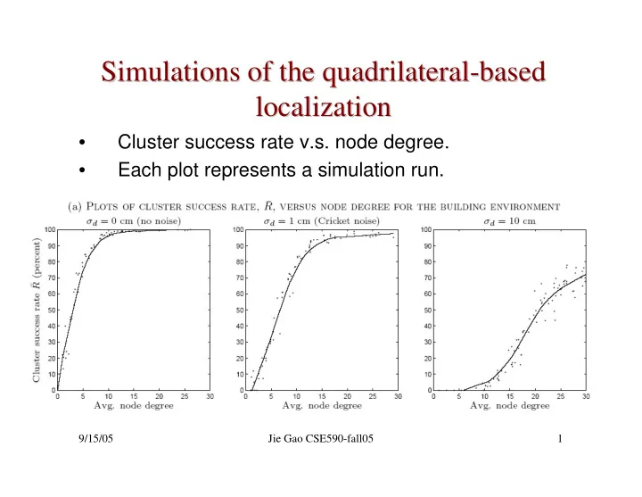
SLIDE 29

9/15/05 Jie Gao CSE590-fall05 29

System challenges System challenges

Physical layer imposes measurement challenges

– Multipath, shadowing, sensor imperfections, changes in propagation properties and more

Extensive computation aspects

– Many formulations of localization problems, how do you solve the

ptimization problem?

– How do you solve the problem in a distributed manner, under computation and storage constraints?

Networking and coordination issues

– Nodes have to collaborate and communicate to solve the problem – If you are using it for routing, it means you don’t have routing support to solve the problem! How do you do it?

System Integration issues

– How do you build a whole system for localization? – How do you integrate location services with other applications? – Different implementation for each setup, sensor, integration issue

SLIDE 30

9/15/05 Jie Gao CSE590-fall05 30

Location Location-

based Routing in

based Routing in Sensor Networks Sensor Networks

Jie Gao

Computer Science Department Stony Brook University

SLIDE 31

9/15/05 Jie Gao CSE590-fall05 31

Papers Papers

[Bose01] P. Bose, P. Morin, I. Stojmenovic and J. Urrutia, Routing

with guaranteed delivery in ad hoc wireless networks, Wireless Networks, 7(6), 609-616, 2001.

[Karp00] Karp, B. and Kung, H.T., Greedy Perimeter Stateless

Routing for Wireless Networks, in MobiCom 2000.

SLIDE 32

9/15/05 Jie Gao CSE590-fall05 32

Routing in ad hoc networks Routing in ad hoc networks

Routing protocols in communication networks obtain route

information between pairs of nodes wishing to communicate.

Proactive protocols: the protocol maintains routing tables at

each node that is updated as changes in the network topology are detected.

Reactive protocols: routes are constructed on demand. No

global routing table is maintained.

Due to the high rate of topology changes, reactive protocols

are more appropriate for ad hoc networks.

– Ad hoc on demand distance vector routing (AODV) – Dynamic source routing (DSR)

However, both depend on flooding for route discovery.

SLIDE 33

9/15/05 Jie Gao CSE590-fall05 33

Geographical routing Geographical routing

“Data-centric” routing: routing is frequently based on a nodes’

attributes and sensed data, rather than on pre-assigned network address.

Geographical routing uses a node’s location to discover path

to that route.

Assumptions:

– Nodes know their geographical location – Nodes know their 1-hop neighbors – Routing destinations are specified geographically (a location, or a geographical region) – Each packet can hold a small amount (O(1)) of routing information. – The connectivity graph is modeled as a unit disk graph.

SLIDE 34

9/15/05 Jie Gao CSE590-fall05 34

Geographical routing Geographical routing

The information that the source node has

– The location of the destination node; – The location of itself and its 1-hop neighbors.

Geographical forwarding: send the packet to the 1-

hop neighbor that makes most progress towards the destination.

– No flooding is involved.

Many ways to measure “progress”.

– The one closest to the destination in Euclidean distance. – The one with smallest angle towards the destination: “compass routing”. – Etc.

SLIDE 35

9/15/05 Jie Gao CSE590-fall05 35

Greedy progress Greedy progress

SLIDE 36

9/15/05 Jie Gao CSE590-fall05 36

Geographical routing may get stuck Geographical routing may get stuck

Geographical routing may stuck at a node whose

neighbors are all further away from the destination than itself.

t s t

?

s

Send packets to the neighbor closest to the destination

SLIDE 37

9/15/05 Jie Gao CSE590-fall05 37

Compass routing may get in loops Compass routing may get in loops

Compass routing may get in a loop.

Send packets to the neighbor with smallest angle towards the destination

SLIDE 38

9/15/05 Jie Gao CSE590-fall05 38

How to get around local minima? How to get around local minima?

Use a planar subgraph: a straight line graph with

no crossing edges. It subdivides the plane into connected regions called faces.

SLIDE 39

9/15/05 Jie Gao CSE590-fall05 39

Face Routing Face Routing

Keep left hand on the wall, walk until hit the straight line

connecting source to destination.

Then switch to the next face.

s t

SLIDE 40

9/15/05 Jie Gao CSE590-fall05 40

Face Routing Face Routing

s t

SLIDE 41

9/15/05 Jie Gao CSE590-fall05 41

Face Routing Face Routing

s t

SLIDE 42

9/15/05 Jie Gao CSE590-fall05 42

Face Routing Face Routing

s t

SLIDE 43

9/15/05 Jie Gao CSE590-fall05 43

Face Routing Face Routing

s t

SLIDE 44

9/15/05 Jie Gao CSE590-fall05 44

Face Routing Face Routing

s t

SLIDE 45

9/15/05 Jie Gao CSE590-fall05 45

Face Routing Face Routing

s t

SLIDE 46

9/15/05 Jie Gao CSE590-fall05 46

Face Routing Face Routing

s t

SLIDE 47

9/15/05 Jie Gao CSE590-fall05 47

All necessary information is stored in the message

– Source and destination positions – The node when it enters the perimeter mode. – The first edge on the current face.

Completely local:

– Knowledge about direct neighbors’ positions is sufficient – Faces are implicit. Only local neighbor ordering around each node is needed

Face Routing Properties Face Routing Properties

“Right Hand Rule”

SLIDE 48

9/15/05 Jie Gao CSE590-fall05 48

What if the destination is disconnected? What if the destination is disconnected?

The perimeter routing will

get back to where it enters the perimeter mode.

Failed – no way to the

destination.

Guaranteed delivery of a

message if there is a path.

SLIDE 49

9/15/05 Jie Gao CSE590-fall05 49

Planar Graph Subtraction Planar Graph Subtraction

Compute a planar subgraph of the unit disk graph.

– Preserves connectivity. – Distributed computation.

SLIDE 50

9/15/05 Jie Gao CSE590-fall05 50

A little detour on A little detour on Delaunay Delaunay triangulation triangulation

SLIDE 51

9/15/05 Jie Gao CSE590-fall05 51

Delaunay Delaunay triangulation triangulation

First proposed by B. Delaunay in 1934.
Numerous applications since then.

SLIDE 52

9/15/05 Jie Gao CSE590-fall05 52

Voronoi Voronoi diagram diagram

Partition the plane into cells such that all the points

inside a cell have the same closest point. Voronoi vertex Voronoi cell Voronoi edge

SLIDE 53

9/15/05 Jie Gao CSE590-fall05 53

Delaunay Delaunay triangulation triangulation

Dual of Voronoi diagram: Connect an edge if their

Voronoi cells are adjacent.

Triangulation of the convex hull.

SLIDE 54

9/15/05 Jie Gao CSE590-fall05 54

Delaunay Delaunay triangulation triangulation

“Empty-circle property”: the circumcircle of a

Delaunay triangle is empty of other points.

The converse is also true: if all the triangles in a

triangulation are locally Delaunay, then the triangulation is a Delaunay triangulation.

SLIDE 55

9/15/05 Jie Gao CSE590-fall05 55

Greedy routing on Greedy routing on Delaunay Delaunay triangulation triangulation

Claim: Greedy routing on DT never gets stuck.

SLIDE 56

9/15/05 Jie Gao CSE590-fall05 56

Delaunay Delaunay triangulation triangulation

For an arbitrary point set, the Delaunay

triangulation may contain long edges.

Centralized construction.
If the nodes are uniformly placed inside a unit disk,

the longest Delaunay edge is O((logn/n)1/3). [Kozma et.al. PODC’04]

Next: 2 planar subgraphs that can be constructed

in a distributed way: relative neighborhood graph and the Gabriel graph.

SLIDE 57

9/15/05 Jie Gao CSE590-fall05 57

Relative Neighborhood Graph and Gabriel Relative Neighborhood Graph and Gabriel Graph Graph

Relative Neighborhood Graph (RNG) contains an

edge uv if the lune is empty of other points.

Gabriel Graph (GG) contains an edge uv if the disk

with uv as diameter is empty of other points.

Both can be constructed in a distributed way.

SLIDE 58

9/15/05 Jie Gao CSE590-fall05 58

Relative Neighborhood Graph and Gabriel Relative Neighborhood Graph and Gabriel Graph Graph

Claim: MST ⊆ RNG ⊆ GG ⊆ Delaunay
Thus, RNG and GG are planar (Delaunay is planar)

and keep the connectivity (MST has the same connectivity of UDG).

SLIDE 59

9/15/05 Jie Gao CSE590-fall05 59

MST MST ⊆ ⊆ RNG RNG ⊆ ⊆ GG GG ⊆ ⊆ Delaunay Delaunay

1. RNG ⊆ GG: if the lune is empty, then the disk with uv as diameter is also empty. 2. GG ⊆ Delaunay: the disk with uv as diameter is empty, then uv is a Delaunay edge.

SLIDE 60

9/15/05 Jie Gao CSE590-fall05 60

MST MST ⊆ ⊆ RNG RNG ⊆ ⊆ GG GG ⊆ ⊆ Delaunay Delaunay

3. MST ⊆ RNG:

Assume uv in MST is not in RNG, there is a

point w inside the lune. |uv|>|uw|, |uv|>|vw|.

Now we delete uv and partition the MST into two

subtrees.

Say w is in the same component with u, then we

can replace uv by wv and get a lighter tree. contradiction. RNG and GG are planar (Delaunay is planar) and keep the connectivity (MST has the same connectivity of UDG).

SLIDE 61

9/15/05 Jie Gao CSE590-fall05 61

An example of UDG An example of UDG

200 nodes randomly deployed in a 2000×2000 meters region. Radio range =250meters

SLIDE 62

9/15/05 Jie Gao CSE590-fall05 62

An example of GG and RNG An example of GG and RNG

GG RNG

SLIDE 63

9/15/05 Jie Gao CSE590-fall05 63

Two problems remain Two problems remain

A subgraph G’ of G is a α-spanner if the shortest

path in G’ is bounded by a constant α times the shortest path length in G.

Both RNG and GG are not spanners a short

path may not exist!

Even if the planar subgraph contains a short path,

can greedy routing and face routing find a short

ne?