Simulation of Rayleigh-Benard Convection on GPUs Massimiliano Fatica - - PowerPoint PPT Presentation

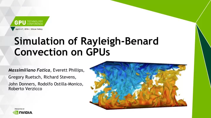
April 4-7, 2016 | Silicon Valley

Massimiliano Fatica, Everett Phillips, Gregory Ruetsch, Richard Stevens, John Donners, Rodolfo Ostilla-Monico, Roberto Verzicco

Simulation of Rayleigh-Benard Convection on GPUs

2

OUTLINE

• Motivation
• AFID Code
• GPU Implementation
• Results
• Conclusions

3

Motivation

• Direct Numerical Simulation (DNS) is an invaluable tool for studying the details of

fluid flows

• DNS must resolve all the flow scales, which requires:
• Computers with large memory (to store variables on large meshes)
• As much computational power as possible (to reduce runtime)
• Time step decreases as mesh is made finer
• Efficient use of parallel machines is essential

4

Motivation

• Current trend in HPC is to use GPUs to increase performance
• Main objectives of this work:
• Port AFiD, a DNS code for RB simulations, to GPU clusters
• Single source code for CPU and GPU versions
• Modify source as little as possible

5

AFiD CODE

6

AFiD Code

High parallel application for Rayleigh-Benard and Taylor-Couette flows Developed by Twente University, SURFSara and University of Rome “Tor Vergata” Open source Fortran 90 + MPI + OpenMP HDF5 with parallel I/O “A pencil distributed finite difference code for strongly turbulent wall-bounded flows”, E. van der Poel, R. Ostilla-Monico, J. Donners, R. Verzicco, Computer & Fluids 116 (2015)

http://www.afid.eu

7

AFiD Code

Navier-Stokes equations with Boussinesq approximation and additional equation for temperature Two horizontal periodic directions (y-z), vertical direction (x) is wall-bounded Mesh is equally spaced in the horizontal directions, stretched in the vertical direction

8

AFiD Code

• Conservative centered finite difference
• Staggered grid
• Fractional step
• Time marching: low-storage RK3 or AB2

(Verzicco and Orlandi, JCP 1996) (Orlandi, Fluid Flow Phenomena)

Numerical scheme

9

Numerical scheme

1) Intermediate non-solenoidal velocity field is calculated using non-linear, viscous, buoyancy and pressure at the current time sub-step At each sub-step: 2) Pressure correction is calculated solving the following Poisson equation 3) The velocity and pressure are then updated using:

AFiD Code

10

AFiD Code

Parallel implementation

• For large Ra numbers (large temperature difference), the implicit integration of

the viscous terms in the horizontal directions becomes unnecessary

• This simplifies the parallel implementation:
• Only the Poisson solver requires global communication
• The code uses a pencil-type decomposition, more general than a slab-type one
• The pencil decomposition is based on the Decomp2D library (www.2decomp.org)

11

AFiD Code

Poisson solver

• The solution of the Poisson equation is always the critical part in incompressible solvers
• Direct solver:
• Fourier decomposition in the horizontal plane
• Tridiagonal solver in the normal direction

(modified wave numbers)

12

AFiD Code

Poisson solver

1) FFT the r.h.s along y – (b) (from real NX x NY x NZ to complex NX x (NY+1)/2 x NZ) 2) FFT the r.h.s. along z – (c) (from complex NX x (NY+1)/2 x NZ to complex NX x (NY+1)/2 x NZ ) 3) Solve tridiagonal system in x for each y and z wavenumber - (a) 4) Inverse FFT the solution along z – (c) (from complex NX x (NY+1)/2 x NZ to complex NX x (NY+1)/2 x NZ ) 5) Inverse FFT the solution along y – (b) (from complex NX x (NY+1)/2 x NZ to real NX x NY x NZ)

13

GPU IMPLEMENTATION

14

Porting Strategy

Since the code is in Fortran 90, natural choices are CUDA Fortran or OpenACC Choice of CUDA Fortran motivated by:

• Personal preference
• Use of CUF kernels made effort comparable to OpenACC
• Explicit data movement is important to optimize CPU/GPU data transfers and network traffic
• Easier to work around compiler/library bugs
• Explicit kernels when/if needed

15

CUDA Fortran

• CUDA is a scalable model for parallel computing
• CUDA Fortran is the Fortran analog to CUDA C

– Program has host and device code similar to CUDA C – Host code is based on the runtime API – Fortran language extensions to simplify data management

• CUDA Fortran implemented in the PGI compilers

16

Kernel Loop Directives (CUF Kernels)

program incTest use cudafor implicit none integer, parameter :: n = 256 integer :: a(n), b integer, device :: a_d(n) a = 1; b = 3; a_d = a !$cuf kernel do <<<*,*>>> do i = 1, n a_d(i) = a_d(i)+b enddo a = a_d if (all(a == 4)) write(*,*) 'Test Passed' end program incTest

Automatic kernel generation and invocation of host code region (arrays used in loops must reside on GPU)

17

Kernel Loop Directives (CUF Kernels)

• Compiler recognizes use of scalar reduction and generates one result

rsum = 0.0 !$cuf kernel do <<<*,*>>> do i = 1, nx rsum = rsum + a_d(i) enddo

• Multidimensional arrays
• Can specify parts of execution parameter

!$cuf kernel do(2) <<< *,* >>> do j = 1, ny do i = 1, nx a_d(i,j) = b_d(i,j) + c_d(i,j) enddo enddo !$cuf kernel do(2) <<<(*,*),(32,4)>>>

18

GPU CODE CPU CODE

Libraries

I/O: HDF5 FFT: FFTW (guru plan) Linear algebra: BLAS+LAPACK Distributed memory: MPI, 2DDecomp with additional x-z and z-x transpose Multicore: OpenMP I/O: HDF5 FFT: CUFFT Linear algebra: custom kernels Distributed memory: MPI, 2DDecomp with improved x-z and z-x transpose Manycore: CUDA Fortran

19

Build System

Original code:

• Build system based on autoconfig
• Double precision enabled with compiler flag

New code:

• Build system based on Makefile
• Single source code for CPU and GPU versions
• Files with .F90 suffix
• Use of preprocessor to enable/guard GPU code
• Explicit control of precision
• Single Makefile to generate both the CPU and GPU binaries (very important to verify results)
• CPU binary can be generated with any compiler ( PGI, Intel, Cray, Gnu)
• GPU binary requires PGI (v15.7 or 16.x)

20

Details

• Variables renaming from modules:

#ifdef USE_CUDA

use cudafor use local_arrays, only: vx => vx_d, vy => vy_d, vz => vz_d #else use local_arrays, only: vx,vy,vz #endif

subroutine ExplicitTermsVX(qcap)

implicit none real(fp_kind), dimension(1:nx,xstart(2):xend(2),xstart(3):xend(3)),intent(OUT) :: qcap #ifdef USE_CUDA attributes(device) :: vx,vy,vz,temp,qcap,udx3c #endif

• F2003 sourced allocation:

allocate(array_b, source=array_a)

• Allocates array_b with the same bounds of array_a
• Initializes array_b with values of array_a
• If array_b is defined with the device attribute, allocation will be on the GPU and host-to-device data transfer occurs
• Use attribute(device):
• Use of generic interfaces:

Interface updateQuantity module procedure updateQuantity_cpu module procedure updateQuantity_gpu end interface updateQuantity

21

Code Example

subroutine CalcMaxCFL(cflm) #ifdef USE_CUDA use cudafor use param, only: fp_kind, nxm, dy => dy_d, dz => dz_d, udx3m => udx3m_d use local_arrays, only: vx => vx_d, vy => vy_d, vz => vz_d #else use param, only: fp_kind, nxm, dy, dz, udx3m use local_arrays, only: vx,vy,vz #endif use decomp_2d use mpih implicit none realintent(out) :: cflm integer :: j,k,jp,kp,i,ip real :: qcf cflm=0.00000001d0 #ifdef USE_CUDA !$cuf kernel do(3) <<<*,*>>> #else !$OMP PARALLEL DO & !$OMP DEFAULT(none) & !$OMP SHARED(xstart,xend,nxm,vz,vy,vx) & !$OMP SHARED(dz,dy,udx3m) & !$OMP PRIVATE(i,j,k,ip,jp,kp,qcf) & !$OMP REDUCTION(max:cflm) #endif do i=xstart(3),xend(3) ip=i+1 do j=xstart(2),xend(2) jp=j+1 do k=1,nxm kp=k+1 qcf=( abs((vz(k,j,i)+vz(k,j,ip))*0.5d0*dz) & +abs((vy(k,j,i)+vy(k,jp,i))*0.5d0*dy) & +abs((vx(k,j,i)+vx(kp,j,i))*0.5d0*udx3m(k))) cflm = max(cflm,qcf) enddo enddo enddo #ifndef USE_CUDA !$OMP END PARALLEL DO #endif call MpiAllMaxRealScalar(cflm) return end subroutine CalcMaxCFL(cflm) #ifdef USE_CUDA use cudafor use param, only: fp_kind, nxm, dy => dy_d, dz => dz_d, udx3m => udx3m_d use local_arrays, only: vx => vx_d, vy => vy_d, vz => vz_d #else use param, only: fp_kind, nxm, dy, dz, udx3m use local_arrays, only: vx,vy,vz #endif use decomp_2d use mpih implicit none real(fp_kind),intent(out) :: cflm integer :: j,k,jp,kp,i,ip real(fp_kind) :: qcf cflm=real(0.00000001,fp_kind) #ifdef USE_CUDA !$cuf kernel do(3) <<<*,*>>> #endif !$OMP PARALLEL DO & !$OMP DEFAULT(none) & !$OMP SHARED(xstart,xend,nxm,vz,vy,vx) & !$OMP SHARED(dz,dy,udx3m) & !$OMP PRIVATE(i,j,k,ip,jp,kp,qcf) & !$OMP REDUCTION(max:cflm) do i=xstart(3),xend(3) ip=i+1 do j=xstart(2),xend(2) jp=j+1 do k=1,nxm kp=k+1 qcf=( abs((vz(k,j,i)+vz(k,j,ip))*real(0.5,fp_kind)*dz) & +abs((vy(k,j,i)+vy(k,jp,i))*real(0.5,fp_kind)*dy) & +abs((vx(k,j,i)+vx(kp,j,i))*real(0.5,fp_kind)*udx3m(k))) cflm = max(cflm,qcf) enddo enddo enddo !$OMP END PARALLEL DO call MpiAllMaxRealScalar(cflm) return end

22

Transpose

1 0 2 3 4 5 1 2 3 4 5 3 1 5 4 2 3 1 5 4 2 1 0 2 3 4 5 1 0 2 3 4 5 1 2 3 4 5 3 1 5 4 2 Original scheme Improved scheme

23

Profiling

Profiling is very important to understand bottlenecks and to spot opportunities for better interaction between the CPU and the GPU For GPU codes, profiling information can be generated with Nvprof and visualized with Nvvp For CPU+GPU codes, it is possible to annotate the profiling timelines using the NVIDIA Tools Extension (NVTX) library NVTX from Fortran and CUDA Fortran:

https://devblogs.nvidia.com/parallelforall/customize-cuda-fortran-profiling-nvtx/

24

NVTX Example

program main use nvtx character(len=4) :: itcount ! First range with standard color call nvtxStartRange("First label”) do n=1,14 ! Create custom label for each marker write(itcount,'(i4)') n ! Range with custom color call nvtxStartRange("Label "//itcount,n) ! Add sleep to make markers big call sleep(1) call nvtxEndRange end do call nvtxEndRange end program main $ pgf90 nvtx.cuf -L/usr/local/cuda/lib –lnvToolsExt $ nvprof -o profiler.output ./a.out NVPROF is profiling process 10653, command: ./a.out Generated result file: /Users/mfatica/profiler.output

25

NVVP Example

40% 20% 25% 15% 15%

26

RESULTS

27

Optimal Configuration

In auto-tuning mode...... factors: 1 2 3 6 9 18 processor grid 1 by 18 time= 0.3238644202550252 processor grid 2 by 9 time= 0.8386047548717923 processor grid 3 by 6 time= 0.9210867749320136 processor grid 6 by 3 time= 0.9363843864864774 processor grid 9 by 2 time= 0.8577810128529867 processor grid 18 by 1 time= 0.5901912318335639 the best processor grid is probably 1 by 18 MPI tasks= 18 ******** CUDA version ******* grid resolution: nx= 1025 ny= 1025 nz= 1025 GPU memory used: 10625.0 - 10832.0 / 11519.6 MBytes GPU memory free: 894.5 - 686.6 / 11519.6 Mbytes Creating initial condition Initial maximum divergence: 0.2818953478714559 Initialization Time = 15.63 sec. WallDt CFL ntime time vmax(1) vmax(2) vmax(3) dmax tempm tempmax tempmin nuslw nussup 0.000 0.000 0 0.000 0.00000E+00 0.00000E+00 0.00000E+00 2.81895E-01 0.00000E+00 0.00000E+00 0.00000E+00 0.00000E+00 0.00000E+00 2.675 0.018 2 0.010 0.00000E+00 1.66194E-03 8.31368E-04 2.04477E-15 4.99492E-01 1.00000E+00 1.30278E-04 1.00000E+00 1.00000E+00 2.747 0.018 3 0.020 0.00000E+00 1.66190E-03 8.31480E-04 2.71691E-16 4.99492E-01 1.00000E+00 1.30276E-04 1.00000E+00 1.00000E+00 2.726 0.018 4 0.030 0.00000E+00 1.66190E-03 8.31655E-04 2.80252E-16 4.99492E-01 1.00000E+00 1.30274E-04 1.00000E+00 1.00000E+00 2.725 0.018 5 0.040 0.00000E+00 1.66193E-03 8.31893E-04 2.84318E-16 4.99492E-01 1.00000E+00 1.30271E-04 1.00000E+00 1.00000E+00

If the 2D processor configuration is not specified as an argument, the code will try to estimate the estimate the optimal configuration GPU code measures the transpose and halo update time

28

Memory Footprint

Memory footprint reduction one of the main goals to increase the mesh size 10243 Computer Time per step GPU #GPUs # nodes Mem. Used (MB) Mem. per GPU (MB) Piz-Daint 1.65s K20X 36 36 5427-5635 5795 Cartesius 2.7s K40 18 9 10625-10832 11519 Latest version Computer Time per step GPU #GPUs # nodes Mem. Used (MB) Mem. per GPU (MB) Piz-Daint 1.7s K20X 32 32 5389-5427 5795 Cartesius 3.18s K40 16 8 10545-10592 11519 1.68s K40 32 16 5415-5463 11519 20483 will fit on Cartesius (SARA) using all the available GPU nodes (64) 40963 will fit on Piz-Daint (CSCS) using 2048 (out of 5272)

29

Performance

Results on Piz-Daint, K20x with 5795MB of memory 2048x3076x3076 Time per step #GPUs Conf

• Mem. Used (MB)

2.4s 640 64x10 5047-5159 1.58s 1024 64x16 3381-3385 0.88s 2048 32x64 1828-1837 0.57s 4096 64x64 1051-1056 1024x1024x1024 Time per step #GPUs Conf

• Mem. Used (MB)

1.7s 32 1x32 5380-5427 0.34s 256 16x16 821-824 0.24s 512 32x16 460-470 0.17s 1024 32x32 322-323

30

Performance

31

Comparison CPU/GPU Code

32

CONCLUSIONS

33

Conclusions

• Port completed
• Excellent speed up and scalability
• Results have been verified to be correct
• The code will be released on Github
• The code will be used to push the boundary of RB simulations

34

Future Work

• Add the multiscale algorithm (finer mesh for temperature equation) to further

reduce the memory footprint

• Split the pencils between CPUs (now completely idle) and GPUs
• Upcoming Pascal GPU with larger memory and improved memory bandwidth will

be very beneficial for this code