Simulating the 4% Universe Hydro-cosmology simulations and data - PowerPoint PPT Presentation

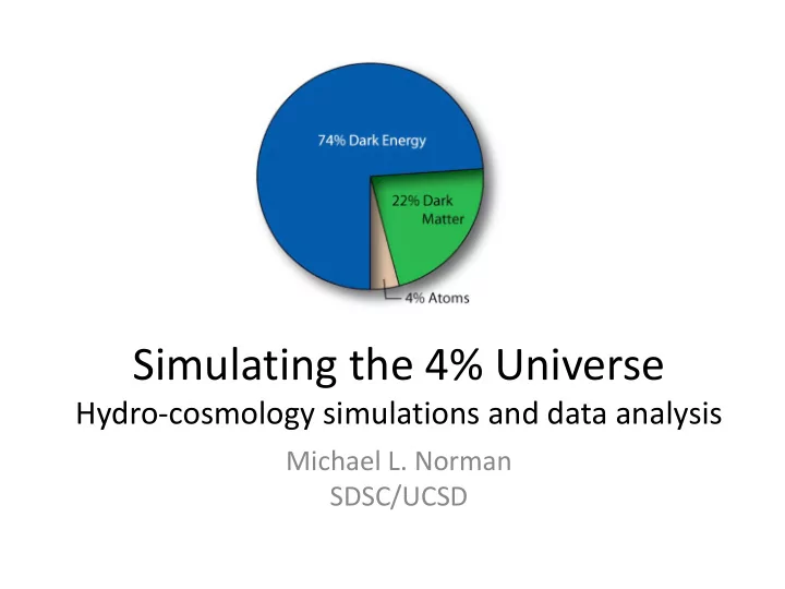
Simulating the 4% Universe Hydro-cosmology simulations and data analysis Michael L. Norman SDSC/UCSD

Lecture Plan • Lecture 1: Hydro-cosmology simulations of baryons in the Cosmic Web – Lyman alpha forest (LAF) – Baryon Acoustic Oscillation (BAO) • Lecture 2: Radiation hydro-cosmology simulations of Cosmic Renaissance – Epoch of Reionization (EOR) – First Galaxies 7/17/2012 ISSAC 2012 SDSC, San Diego, USA 2

Motivation • It’s the part of the Universe we can see • Involves real astrophysics which is complicated and interesting • Can place constraints on the dark universe • Computational discoveries Norman (1997) 7/17/2012 ISSAC 2012 SDSC, San Diego, USA 3

Computational Discoveries • Physical nature of Lyman alpha forest absorption systems Cen+1994, Zhang+1995, Hernquist+1996 • Existence of the warm-hot intergalactic medium Cen & Ostriker 1999 • Mass scale of Pop III stars Abel+2001, Bromm+2002 7/17/2012 ISSAC 2012 SDSC, San Diego, USA 4

What is Hydro-cosmology? = + dark matter ideal gas dynamics hydrodynamic + + cosmology gravity “microphysics” 7/17/2012 ISSAC 2012 SDSC, San Diego, USA 5

1990 adiabatic gas dynamics 7/17/2012 ISSAC 2012 SDSC, San Diego, USA 6

1990 adiabatic gas dynamics 7/17/2012 ISSAC 2012 SDSC, San Diego, USA 7

1991 gas dynamics + radiative cooling 7/17/2012 ISSAC 2012 SDSC, San Diego, USA 8

Baryons! (not the Bolshoi simulation) 7/17/2012 ISSAC 2012 SDSC, San Diego, USA 9

http://enzo-project.org 7/17/2012 ISSAC 2012 SDSC, San Diego, USA 10

http://hipacc.ucsc.edu/html/2010SummerSchool_archive.html 7/17/2012 ISSAC 2012 SDSC, San Diego, USA 11

LECTURE 1 Hydro-cosmology simulations of baryons in the cosmic web *** (Lyman α forest) 7/17/2012 ISSAC 2012 SDSC, San Diego, USA 12

Q: Where are the baryons? A: In the IGM mostly IGM Cen & Ostriker (1999) 7/17/2012 ISSAC 2012 SDSC, San Diego, USA 13

Observing the intergalactic medium in quasar absorption line spectra Lyman α forest Source: M. Murphy 7/17/2012 ISSAC 2012 SDSC, San Diego, USA 14

High Resolution Spectrum virtually every absorption line is H Ly α Kirkman & Tytler (1997) at a different redshift along the LOS 7/17/2012 ISSAC 2012 SDSC, San Diego, USA 15

Physical Origin of the Lyman Alpha Forest Cen et al. 1994, Zhang et al. 1995, Hernquist et al. 1996 “The Cosmic Web” • intergalactic medium exhibits cosmic web structure at high z • models explain observed hydrogen absorption spectra 5 Mpc/h N=128 3 Zhang, Anninos, Norman (1995) 7/17/2012 ISSAC 2012 SDSC, San Diego, USA

Ly α absorption directly probes DM distribution Zhang et al. (1998) 7/17/2012 ISSAC 2012 SDSC, San Diego, USA 17

Cosmology from the Ly α Forest • What is measured • The standard model • Observations vs. simulations I: – spectacular agreement at the ~10% level • DM power spectrum estimation • Observations vs. simulations II: – discrepancies at the 1-2% level 7/17/2012 ISSAC 2012 SDSC, San Diego, USA 18

The Standard Model • Your favorite cosmological model ( Ω dm , Ω b , Ω Λ , H 0 , σ 8 , n s ) • IGM of primordial H and He photoionized by homogeneous but evolving UVB due to GALS and QSOs (J UVB (z)) • Ly α forest due to optically thin absorption in highly ionized gas in intergalactic filaments tracing the DM distribution • LLS and DLAs due to optically thick absorption in denser ionized gas in halos 7/17/2012 ISSAC 2012 SDSC, San Diego, USA 19

What is Observed Kirkman & Tytler (1997) 7/17/2012 ISSAC 2012 SDSC, San Diego, USA 20

And hundreds more… 7/17/2012 ISSAC 2012 SDSC, San Diego, USA 21

Simulated Spectra and Fitting Zhang et al. (1997) 7/17/2012 ISSAC 2012 SDSC, San Diego, USA 22

Observations vs. Simulations I. Remarkable Agreement on Line Statistics Kirkman & Tytler (1997) <b> = 23 σ = 14 7/17/2012 23 Zhang, Anninos, Norman (1995)

What is a Ly α Forest Absorber? LAF 7/17/2012 ISSAC 2012 SDSC, San Diego, USA 24 Zhang, Anninos, Meiksin & Norman (1998)

What is a Ly α Forest Absorber? Z=3 7/17/2012 ISSAC 2012 SDSC, San Diego, USA 25 Zhang, Anninos, Meiksin & Norman (1998)

What is a Ly α Forest Absorber? • Sheet or filament of low overdensity relative to the local mean λ Jeans • Not gravitationally bound in 3D • Unbiased WRT to dark matter • Photo-ionized gas at λ Jeans ~10 4 K • D ~ λ Jeans ~ 100 kpc 7/17/2012 ISSAC 2012 SDSC, San Diego, USA 26 Zhang, Anninos, Meiksin & Norman (1998)

Resolving the Ly α Forest Bryan, Machacek, Anninos, Norman (1999) • Observed linewidths reflect – Thermal broadening – Hubble broadening (redshift, LOS, and N HI dependent) – Possibly turbulent broadening • Simulated linewidths reflect above plus – Numerical resolution broadening 7/17/2012 ISSAC 2012 SDSC, San Diego, USA 28

Higher resolution simulations predict lines that are too narrow Bryan et al. (1999) 7/17/2012 ISSAC 2012 SDSC, San Diego, USA 29

Higher resolution simulations predict lines that are too narrow • Possible reasons – Cosmological model wrong – UV background model wrong – Box too small (large scale power missing) – Missing heat sources (He II reionization, X-rays, …) – Missing turbulent broadening (galactic winds?) – Magnetic support? 13 years later, this discrepancy has not been resolved  Opportunity for a fundamental contribution 7/17/2012 ISSAC 2012 SDSC, San Diego, USA 30

Jena et al. (2005) • 40 fully hydrodynamic simulations* varying – Cosmological parameters – Box size N=1024 3 – Numerical resolution L = 80 Mpc – UV background intensity Baryon Overdensity, z=3 – Extra heating put in by hand • Sensitivity analysis and uncertainty quantification • Observations  Concordance model @z=1.95 *Data available at http://lca.ucsd.edu/data/concordance/ 7/17/2012 ISSAC 2012 SDSC, San Diego, USA 31

Sensitivity analysis and uncertainty quantification • Derive simple parametric fits that connect key inputs to output • Key inputs – σ 8 : amplitude of matter fluctuations – γ 912 : normalized HI photoionization rate – X 228 : normalized HeII photoheating rate – L: simulation box size – C: cell resolution • Key outputs – <F>=exp(- τ eff ): mean transmitted flux – b σ : median Doppler width – P -2 , P -1.5 , P -1 : flux power at log k =10 -2 , 10 -1.5 , 10 -1 s/km 7/17/2012 ISSAC 2012 SDSC, San Diego, USA 32

Flux Power υ − ( ) f f δ υ ≡ ( ) ; f is mean flux for spectrum f f = δ δ δ δ υ ( ) ( ) * ( ); ( ) is 1D FT of ( ) P k k k k f f f f f P -2 P -1.5 P -1 OBS SIMS Jena et al. (2005) 7/17/2012 ISSAC 2012 SDSC, San Diego, USA 33

Table of Simulations 7/17/2012 ISSAC 2012 SDSC, San Diego, USA 34

Table of Simulations, cont’d 7/17/2012 ISSAC 2012 SDSC, San Diego, USA 35

Scaling Relations b σ before scaling after scaling τ eff Jena et al. (2005) 7/17/2012 ISSAC 2012 SDSC, San Diego, USA 36

Findings • After scaling out boxsize and resolution effects, a wide range of σ 8 (0.8< σ 8 <1.1) fit observations (<F>, b σ , P -1 ) by adjusting γ 912 and X 228 • Using only <F>, b σ , P -1 cannot uniquely determine σ 8 , γ 912 , X 228 because b σ and P -1 are correlated • Using <F> to fix γ 912, then σ 8 and X 228 degenerate Jena et al. (2005) 7/17/2012 ISSAC 2012 SDSC, San Diego, USA 37

Findings (cont’d) • Can potentially remove degeneracy using large scale flux power P -2 • This was not explored in Jena+(2005) – box sizes too small – observational uncertainties at low k • Based on scalings, need at least 100 Mpc boxes and at least 50 kpc resolution  2000 3 but preferably 25 kpc  4000 3 • Comparable to largest N-body simulations, but without the need to resolve halo substructure – Eulerian simulations on uniform grids are adequate 7/17/2012 ISSAC 2012 SDSC, San Diego, USA 38

a 4096 3 hydro-cosmology simulation L=614 Mpc, Cell=150 kpc 7/17/2012 ISSAC 2012 SDSC, San Diego, USA 39

7/17/2012 ISSAC 2012 SDSC, San Diego, USA 40

Estimating P(k) from SDSS Quasars McDonald et al. (2005) = 2 • Key ansatz: P ( k , z ) b ( k ) P ( k , z ) F M • Where bias b(k) is determined from hydro simulations (Croft et al. 1998, 2002) • Difficulty with SDSS spectra is that lines are not resolved, and therefore P F (k) needs to be corrected for many systematics errors – Continuum level -- Noise – Metal line contamination -- UVB fluctuations – High column density absorbers • In practice, b(k) is estimated on large scales from non- hydrodynamic simulations of the LAF that model the absorption phenomenologically • UPSHOT: lots of systematic uncertainties 7/17/2012 ISSAC 2012 SDSC, San Diego, USA 41

Observations vs. Simulations II. Tytler et al. (2009) • Revisit Jena et al. (2005) suite of simulations with more analysis on the effect of box size on LAF observables, incl. P F (k) • All parameters except L kept constant (incl. resolution) • Bigger box means: – More total power – Higher peak densities – Higher peculiar velocities – Hotter gas 7/17/2012 ISSAC 2012 SDSC, San Diego, USA 42