
SLIDE 1
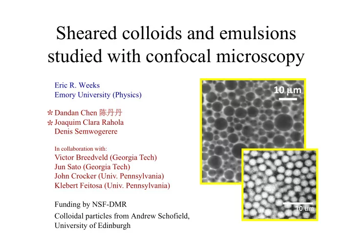
Sheared colloids and emulsions studied with confocal microscopy
Eric R. Weeks Emory University (Physics) Dandan Chen 陈丹丹 Joaquim Clara Rahola Denis Semwogerere
In collaboration with:Victor Breedveld (Georgia Tech) Jun Sato (Georgia Tech) John Crocker (Univ. Pennsylvania) Klebert Feitosa (Univ. Pennsylvania) Funding by NSF-DMR Colloidal particles from Andrew Schofield, University of Edinburgh
* *