Session topics The plane sweep paradigm Visibility of a point - - PDF document

1

Yaron Ostrovsky-Berman, Computational Geometry, Spring 2005

1

Computational Geometry

Exercise session #3

Yaron Ostrovsky-Berman, Computational Geometry, Spring 2005

2

Session topics

• The plane sweep paradigm
• Visibility of a point

Problem description and motivation Solution with a rotating sweepline

• Maxima of a point set
• Homework number 2

Yaron Ostrovsky-Berman, Computational Geometry, Spring 2005

3

The plane sweep paradigm

• Sweep the plane with a line, maintain the

status of the line, update it at scheduled event points, and maintain the sweep invariant.

• Details are problem-dependent, but general

approach is similar to all sweep algorithms.

• Required data structures:

The event structure The status structure The invariant structure (partial problem solution)

Yaron Ostrovsky-Berman, Computational Geometry, Spring 2005

4

Example: line segment intersection

• Events

Endpoints of segments or detected intersection points. DAST: a balanced binary search tree ordered according to y coordinate (x coordinate breaks ties)

• Status

Segments intersection by horizontal line at current y coordinate. DAST: a balanced binary search tree according to segment

• rder on horizontal line.
• Invariant

All intersection points above line were reported. DAST: list of reported intersection points.

Yaron Ostrovsky-Berman, Computational Geometry, Spring 2005

5

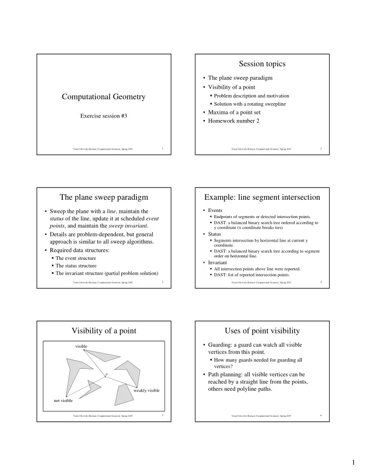
Visibility of a point

visible not visible weakly visible

p

Yaron Ostrovsky-Berman, Computational Geometry, Spring 2005

6

Uses of point visibility

• Guarding: a guard can watch all visible

vertices from this point.

How many guards needed for guarding all vertices?

• Path planning: all visible vertices can be

reached by a straight line from the points,

• thers need polyline paths.

2

Yaron Ostrovsky-Berman, Computational Geometry, Spring 2005

7

Computing the visible vertices

ρ

Yaron Ostrovsky-Berman, Computational Geometry, Spring 2005

8

Rotational sweepline

• Events:

Vertices of obstacles sorted CCW around point. DAST: sorted list or array.

• Status:

Edges of obstacles intersecting ρ. DAST: balanced binary search tree ordered according to intersection with ρ.

• Invariant:

All vertices with angle between horizontal segment and ρ have been determined for visibility. DAST: lists of visible and invisible vertices.

Yaron Ostrovsky-Berman, Computational Geometry, Spring 2005

9

Algorithm outline

• Input: a set S of polygonal obstacles and a point p that does not lie on the

interior of any obstacle.

• Output: set of all vertices visible from p.

1. Sort obstacle vertices in CCW according to angle with positive x

• direction. In case of ties, sort by increasing distance to p. Let w1,…,wn be

sorted list of events. 2. Initialize ρ at positive x direction. 3. Find obstacle edges intersected by ρ and inset them in status tree T

• rdered by intersection distance from p.

4. Initialize output W to {}. 5. For i=1 to n do 1. If Visible(wi) then add wi to W 2. Insert into T obstacle edges incident to wi that are left of line from p to wi 3. Delete from T obstacle edges incident to wi that are right of line from p to wi 6. Return W

Yaron Ostrovsky-Berman, Computational Geometry, Spring 2005

10

Cases where ρ contains multiple vertices

wi-1 wi

p

wi-1 wi

p

wi-1 wi

p

wi-1 wi

p

Yaron Ostrovsky-Berman, Computational Geometry, Spring 2005

11

Checking for visibility

Subroutine Visible(wi)

1. If [pwi] intersects the interior of the obstacle of which wi is a vertex, return false 2. Else if i=1or wi-1 is not on segment [pwi]

• Search in T for edge e in leftmost leaf.
• If e exists and [pwi] intersects e then return false
• Else return true

3. Else if wi-1 is not visible return false 4. Else

• Search in T for edge e that intersects [wi-1wi]
• If e exists then return false
• Else return true

Yaron Ostrovsky-Berman, Computational Geometry, Spring 2005

12

Complexity analysis

• Data structures are linear in number of
• bstacle vertices n.
• Initial angular sorting takes O(nlogn) time.
• Number of events: n.
• Searching T for intersection: O(logn) time.
• Status update operations take O(logn) time

each.

• Overall: O(n) space and O(nlogn) time.

3

Yaron Ostrovsky-Berman, Computational Geometry, Spring 2005

13

Variations of visibility problems

Visibility region in simple polygon Edge visibility

Yaron Ostrovsky-Berman, Computational Geometry, Spring 2005

14

Maxima of a point set

• Definition: point p dominates point q (denoted

p >> q or q << p) if for i=1,…,d we have pi≥qi (the relation << is called dominance).

• Definition: A point p is S is called a maximal

element (or maximum) if there does not exist q in S such that q >> p.

• Problem: find all the maxima of a point set

under the dominance condition.

Yaron Ostrovsky-Berman, Computational Geometry, Spring 2005

15

Relation to convex hulls

x1 x2 (++) (-+) (--) (+-)

Yaron Ostrovsky-Berman, Computational Geometry, Spring 2005

16

Lower bound on complexity

• Reduction from sorting to maxima finding.
• Sorting input: x1,…,xn
• Linear time reduction:

S = {pi=(xi,yi)|xi+yi=const}

• From construction: xi < xj <==> yi > yj
• All the points are maxima!
• To determine that pi is maximal, any algorithm must

conclude that there is no j≠i s.t. xi < xj and yi < yj ==>

• For all j≠i either xi > xj or yi > yj, that is xi > xj or xj > xi
• For each pair {xi,xj} relative ordering of elements

known ==> solution to sorting problem.

Yaron Ostrovsky-Berman, Computational Geometry, Spring 2005

17

Computing maxima with sweepline

• Events:

Intersection of horizontal line with input point. DAST: queue of points, sorted by decreasing y.

• Status:

Right-most point passed so far in sweep. DAST: x coordinate of rightmost point.

• Invariant:

All maxima points above line discovered. DAST: list of maxima points.

• Complexity: dominated by sorting: O(nlogn)

Yaron Ostrovsky-Berman, Computational Geometry, Spring 2005

18

Generalization to 3D (sweep plane)

• All points below plane are dominated in the x3

coordinate.

• Status structure: projection to the x1-x2 plane of

points which are maxima above current plane position.

• The idea: project current event point p into x1-

x2 plane and check if dominated by points in status.

If dominated, then continue, else update status by removing points dominated by p, and adding p.

4

Yaron Ostrovsky-Berman, Computational Geometry, Spring 2005

19

Query and update of status structure

x1 x2

p

successorx1(p) successorx2(p)

Yaron Ostrovsky-Berman, Computational Geometry, Spring 2005

20

Complexity of space-sweep

• Status maintained as a balanced search tree on

the x1 coordinate.

• Exactly n events to handle.
• Each event has a O(logn) query time, and

possible update operations on structure.

• A maximum of n deletions from structure,

each costing O(logn) time.

• Overall complexity: O(n) space and O(nlogn)

time.

Yaron Ostrovsky-Berman, Computational Geometry, Spring 2005

21

Remarks

• The space sweep appraoch fails for dimensions

higher than 3.

• With a clever divide & conquer algorithm, the

problem is solved for dimension d≥2 in O(n(logn)d-2 + nlogn) time [Preparat & Shamos, page 155-159]