
SLIDE 1
April 24, 2008 CSSE/MA 325 Lecture #25 1
Session overview
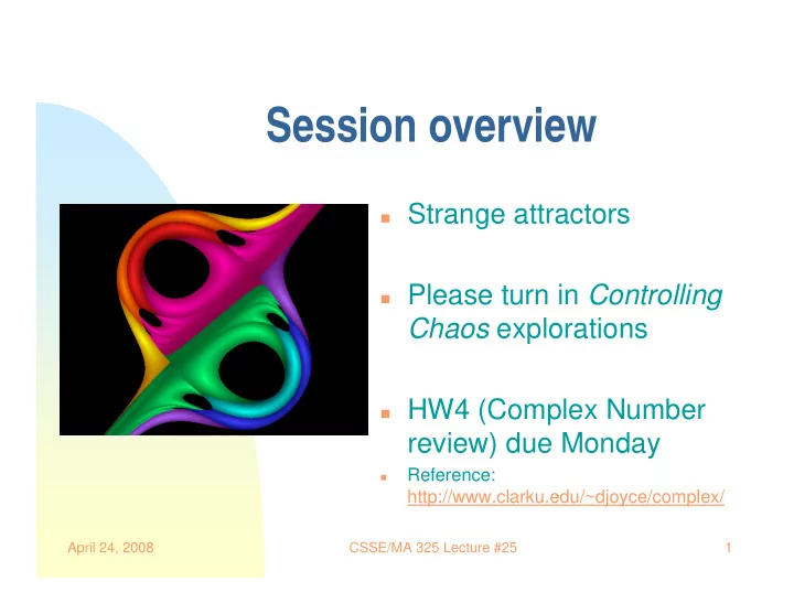
Strange attractors Please turn in Controlling
Chaos explorations
HW4 (Complex Number
review) due Monday
- Reference:
http://www.clarku.edu/~djoyce/complex/