Serious Microfoundations High MPC The Distribution of Wealth and - PowerPoint PPT Presentation

“Serious” Microfoundations ⇒ High MPC The Distribution of Wealth and the Marginal Propensity to Consume Defining ‘the MPC’ ( ≡ κ )? If households receive a surprise extra 1 unit of income, Christopher Carroll 1 Jiri Slacalek 2 Kiichi Tokuoka 3 Matthew N. White 4 how much will be in aggregate spent over the next year? 1 Johns Hopkins University and NBER Elements that interact with each other to produce the result: ccarroll@jhu.edu ◮ Households are heterogeneous 2 European Central Bank jiri.slacalek@ecb.int ◮ Wealth is unevenly distributed 3 Ministry of Finance, Japan ◮ c function is highly concave kiichi.tokuoka@mof.go.jp ◮ ⇒ Distributional issues matter for aggregate C 4 University of Delaware Giving 1 to the poor � = giving 1 to the rich mnwecon@udel.edu 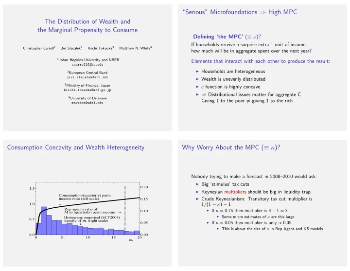Consumption Concavity and Wealth Heterogeneity Why Worry About the MPC ( ≡ κ )? Nobody trying to make a forecast in 2008–2010 would ask: ◮ Big ‘stimulus’ tax cuts 0.20 1.5 ◮ Keynesian multipliers should be big in liquidity trap Consumption �� quarterly � perm ◮ Crude Keynesianism: Transitory tax cut multiplier is income ratio � left scale � 0.15 1.0 1 / (1 − κ ) − 1 � Rep agent's ratio of ◮ If κ = 0 . 75 then multiplier is 4 − 1 = 3 0.10 M to � quarterly � perm income � ◮ Some micro estimates of κ are this large Histogram: empirical � SCF2004 � 0.5 density of � � � right scale � ◮ If κ = 0 . 05 then multiplier is only ≈ 0 . 05 0.05 � ◮ This is about the size of κ in Rep Agent and KS models 0.0 0.00 0 5 10 15 20 � �

Microeconomics of Consumption Our Goal: “Serious” Microfoundations Requires three changes to well-known Krusell–Smith (1998) model: Since Friedman’s (1957) PIH: ◮ c chosen optimally: 1. Sensible microeconomic income process: Friedman Goal: smooth c in light of beliefs about y fluctuations 2. Finite lifetimes: Blanchard ◮ Single most important thing to get right is income dynamics! 3. Match wealth distribution ◮ With smooth c , income dynamics drive everything! ◮ Here, achieved by preference heterogeneity ◮ View it as a proxy for many kinds of heterogeneity ◮ Saving/dissaving: Depends on whether E [∆ y ] ↑ or E [∆ y ] ↓ ◮ Age ◮ Wealth distribution depends on integration of saving ◮ Optimism/Pessimism about Growth ◮ Cardinal sin: Assume crazy income dynamics ◮ Risk aversion ◮ Throws out the defining core of the intellectual framework ◮ Rate of Return ◮ . . . To-Do List Friedman (1957): Permanent Income Hypothesis 1. Calibrate realistic income process = P t + T t Y t 2. Match empirical wealth distribution C t = P t 3. Back out optimal C and MPC out of transitory income 4. Is MPC in line with empirical estimates? Progress since then ◮ Micro data: Friedman description of income shocks works well Our Question: ◮ Math: Friedman’s words well describe optimal solution to Does a model that matches micro facts about income dynamics and wealth distribution give different (and more plausible) answers dynamic stochastic optimization problem of impatient than KS to macroeconomic questions (say, about the response of consumers with geometric discounting under CRRA utility consumption to fiscal ‘stimulus’)? with uninsurable idiosyncratic risk calibrated using these micro income dynamics (!)

Our (Micro) Income Process Further Details of Income Process Idiosyncratic (household) income process is logarithmic Friedman: Modifications from Carroll (1992) Transitory income ξ t incorporates unemployment insurance: y t +1 = p t +1 ξ t +1 W p t +1 = p t ψ t +1 ξ t = µ with probability u (1 − τ )¯ = ℓθ t with probability 1 − u p t = permanent income ξ t = transitory income µ is UI when unemployed ψ t +1 = permanent shock τ is the rate of tax collected for the unemployment benefits W = aggregate wage rate Model Without Aggr Uncertainty: Decision Problem What Happens After Death? � � ψ 1 − ρ u + β � v ( m t ) = max D E t t +1 v ( m t +1 ) { c t } ◮ You are replaced by a new agent whose permanent income is s.t. equal to the population mean = m t − c t a t ◮ Prevents the population distribution of permanent income a t ≥ 0 from spreading out a t / ( � = D ψ t +1 ) k t +1 m t +1 = ( � + r ) k t +1 + ξ t +1 α Z ( K / ¯ ℓ L ) α − 1 r = (State and control variables normalized by p t W)

Ergodic Distribution of Permanent Income Parameter Values Exists, if death eliminates permanent shocks: ◮ β , ρ , α , δ , ¯ ℓ , µ , and u taken from JEDC special volume ◮ Key new parameter values: D E [ ψ 2 ] < 1 . � Holds. Description Param Value Source Population mean of p 2 : Prob of Death per Quarter D 0 . 00625 Life span of 40 years σ 2 Carroll (1992) ; SCF Variance of Log ψ t 0 . 016 / 4 ψ D DeBacker et al. (2013) M [ p 2 ] = D E [ ψ 2 ] σ 2 Carroll (1992) 1 − � Variance of Log θ t 0 . 010 × 4 θ Annual Income, Earnings, or Wage Variances Typology of Our Models—Four Dimensions 1. Discount Factor β σ 2 σ 2 ψ ξ Our parameters 0 . 016 0 . 010 ◮ ‘ β -Point’ model: Single discount factor ◮ ‘ β -Dist’ model: Uniformly distributed discount factor Carroll (1992) 0 . 016 0 . 010 Storesletten, Telmer, and Yaron (2004) 0 . 008–0 . 026 0 . 316 2. Aggregate Shocks Meghir and Pistaferri (2004) ⋆ 0 . 031 0 . 032 ◮ (No) Low, Meghir, and Pistaferri (2010) 0 . 011 − ◮ Krusell–Smith Blundell, Pistaferri, and Preston (2008) ⋆ 0 . 010–0 . 030 0 . 029–0 . 055 ◮ Friedman/Buffer Stock DeBacker, Heim, Panousi, Ramnath, and Vidangos (2013) 0 . 007–0 . 010 0 . 15–0 . 20 3. Empirical Wealth Variable to Match Implied by KS-JEDC 0 . 0 . 038 Implied by Castaneda et al. (2003) 0 . 03 0 . 006 ◮ Net Worth ◮ Liquid Financial Assets ⋆ Meghir and Pistaferri (2004) and Blundell, Pistaferri, and Preston (2008) assume that the transitory component 4. Life Cycle is serially correlated (an MA process), and report the variance of a subelement of the transitory component. σ 2 ξ for ◮ Perpetual Youth (a la Blanchard) ◮ Overlapping Generations these articles are calculated using their MA estimates.

Dimension 1: Estimation of β -Point and β -Dist Results: Wealth Distribution ‘ β -Point’ model � 1 ◮ ‘Estimate’ single ` β by matching the capital–output ratio KS � JEDC Β� Point 0.75 ‘ β -Dist’ model—Heterogenous Impatience Β� Dist US data � SCF � ◮ Assume uniformly distributed β across households 0.5 KS � Hetero ◮ Estimate the band [` β − ∇ , ` β + ∇ ] by minimizing distance between model ( w ) and data ( ω ) net worth held by the top 20, 40, 60, 80% 0.25 ( w i − ω i ) 2 , � min { ` β, ∇} i =20 , 40 , 60 , 80 0 25 50 75 100 s.t. aggregate net worth–output ratio matches the steady-state value Percentile from the perfect foresight model Results: Wealth Distribution Marginal Propensity to Consume & Net Worth Micro Income Process KS-Orig ⋄ Friedman/Buffer Stock KS-JEDC � 0.6 � � Most Impatient � left scale � � 1.5 Point Uniformly Our solution Hetero 0.5 Discount Distributed Identical Patience � left scale � � Factor ‡ Discount 0.4 1.0 Factors ⋆ U.S. Data ∗ 0.3 β -Point β -Dist � Most Patient � left scale � Rep agent's ratio of Top 1% 10.1 26.7 2.6 3.0 24.0 29.6 0.2 0.5 M to � quarterly � perm income � Top 20% 54.8 83.3 35.9 35.0 88.0 79.5 Histogram: empirical density of 0.1 Top 40% 76.4 94. 60.1 92.9 net worth � right scale � � Top 60% 89.6 97.6 78.5 98.7 0.0 0.0 0 5 10 15 20 Top 80% 97.4 99.4 92. 100.4 � � Notes: ‡ : ` β = 0 . 9894. ⋆ : ( ` β, ∇ ) = (0 . 9867 , 0 . 0067). Bold points are targeted. K t / Y t = 10 . 3.