[PPT] - Sequence alignment Alignment specifies which positions in two PowerPoint Presentation

SLIDE 1

Introduction to bioinformatics, Autumn 2007 41

Sequence alignment

l

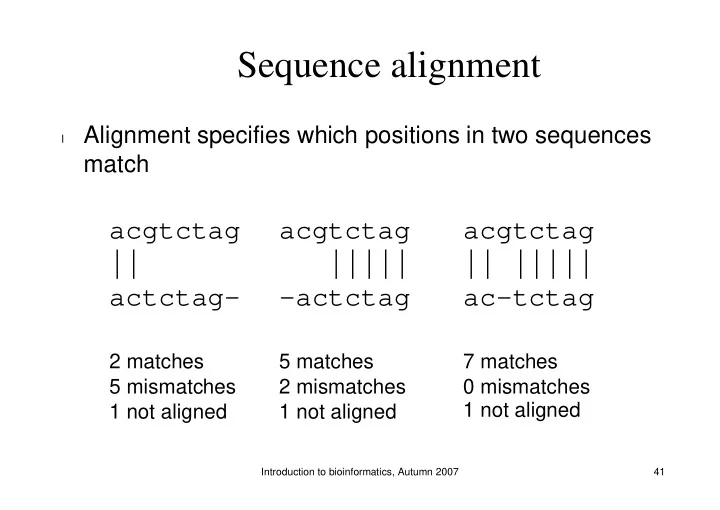
Alignment specifies which positions in two sequences match

acgtctag |||||

actctag

5 matches 2 mismatches 1 not aligned

acgtctag || actctag-

2 matches 5 mismatches 1 not aligned

acgtctag || ||||| ac-tctag

7 matches 0 mismatches 1 not aligned

SLIDE 2

Introduction to bioinformatics, Autumn 2007 42

Mutations: Insertions, deletions and substitutions

l

Insertions and/or deletions are called indels

− We can’t tell whether the ancestor sequence had a base or

not at indel position

acgtctag |||||

actctag

Indel: insertion or deletion of a base with respect to the ancestor sequence Mismatch: substitution (point mutation) of a single base

SLIDE 3

Introduction to bioinformatics, Autumn 2007 43

Problems

l

What sorts of alignments should be considered?

l

How to score alignments?

l

How to find optimal or good scoring alignments?

l

How to evaluate the statistical significance of scores? In this course, we discuss each of these problems briefly. Course Biological sequence analysis tackles all four in- depth.

SLIDE 4

Introduction to bioinformatics, Autumn 2007 44

Sequence Alignment (chapter 6)

l

The biological problem

l

Global alignment

l

Local alignment

l

Multiple alignment

SLIDE 5

Introduction to bioinformatics, Autumn 2007 45

Global alignment

l

Problem: find optimal scoring alignment between two sequences (Needleman & Wunsch 1970)

l

Every position in both sequences is included in the alignment

l

We give score for each position in alignment

− Identity (match) +1 − Substitution (mismatch) -µ − Indel

l

Total score: sum of position scores WHAT || WH-Y

S(WHAT/WH-Y) = 1 + 1 – – µ

SLIDE 6

Introduction to bioinformatics, Autumn 2007 46

Dynamic programming

l

How to find the optimal alignment?

l

We use previous solutions for optimal alignments of smaller subsequences

l

This general approach is known as dynamic programming

SLIDE 7

Introduction to bioinformatics, Autumn 2007 47

Introduction to dynamic programming: the money change problem

l

Suppose you buy a pen for 4.23€ and pay for with a 5€ note

l

You get 77 cents in change – what coins is the cashier going to give you if he or she tries to minimise the number of coins?

l

The usual algorithm: start with largest coin (denominator), proceed to smaller coins until no change is left:

− 50, 20, 5 and 2 cents

l

This greedy algorithm is incorrect, in the sense that it does not always give you the correct answer

SLIDE 8

Introduction to bioinformatics, Autumn 2007 48

The money change problem

How else to compute the

change?

We could consider all possible

ways to reduce the amount of change

Suppose we have 77 cents

change, and the following coins: 50, 20, 5 cents

We can compute the change

with recursion

Figure shows the recursion

tree for the example 77 72 27 57 7 22 7 37 52 22 52 67 …

50 20 5

Many values are computed

more than once!

This leads to a correct but

very inefficient algorithm

SLIDE 9

Introduction to bioinformatics, Autumn 2007 49

The money change problem

l

We can speed the computation up by solving the change problem for all i n

− Example: solve the problem for 9 cents with available coins

being 1, 2 and 5 cents

l

Solve the problem in steps, first for 1 cent, then 2 cents, and so on

l

In each step, utilise the solutions from the previous steps

SLIDE 10

Introduction to bioinformatics, Autumn 2007 50

The money change problem

1 2 3 4 5 6 7 8 9

Amount of change left

l

Algorithm runs in time proportional to Md, where M is the amount of change and d is the number of coin types

l

The same technique of storing solutions of subproblems can be utilised in aligning sequences

SLIDE 11

Introduction to bioinformatics, Autumn 2007 51

Representing alignments and scores

X Y X X H X W

T

A H W

WHAT

|| WH-Y

Alignments can be represented in the following tabular form. Each alignment corresponds to a path through the table.

SLIDE 12

Introduction to bioinformatics, Autumn 2007 52

Y H W

T

A H W

WHAT

|| WH-Y Global alignment score S3,4 = 2--µ

2--µ 2-

2 1

Representing alignments and scores

SLIDE 13

Introduction to bioinformatics, Autumn 2007 53

Filling the alignment matrix

Y H W

T

A H W

Case 1

Case 2 Case 3

Consider the alignment process at shaded square. Case 1. Align H against H (match or substitution). Case 2. Align H in WHY against – (indel) in WHAT. Case 3. Align H in WHAT against – (indel) in WHY.

SLIDE 14

Introduction to bioinformatics, Autumn 2007 54

Filling the alignment matrix (2)

Y H W

T

A H W

Case 1

Case 2 Case 3

Scoring the alternatives. Case 1. S2,2 = S1,1 + s(2, 2) Case 2. S2,2 = S1,2 Case 3. S2,2 = S2,1 s(i, j) = 1 for matching positions, s(i, j) = - µ for substitutions. Choose the case (path) that yields the maximum score. Keep track of path choices.

SLIDE 15

Introduction to bioinformatics, Autumn 2007 55

Global alignment: formal development

A = a1a2a3…an, B = b1b2b3…bm

a3 a2 a1

b4

b3 b2 b1

3

2 1 4 3 2 1 b1 b2 b3 b4

a1

a2 a3

l Any alignment can be written

as a unique path through the matrix

l Score for aligning A and B up

to positions i and j: Si,j = S(a1a2a3…ai, b1b2b3…bj)

SLIDE 16

Introduction to bioinformatics, Autumn 2007 56

Scoring partial alignments

l

Alignment of A = a1a2a3…an with B = b1b2b3…bm can end in three ways

− Case 1: (a1a2…ai-1) ai

(b1b2…bj-1) bj

− Case 2: (a1a2…ai-1) ai

(b1b2…bj) -

− Case 3: (a1a2…ai) –

(b1b2…bj-1) bj

SLIDE 17

Introduction to bioinformatics, Autumn 2007 57

Scoring alignments

l

Scores for each case:

− Case 1: (a1a2…ai-1) ai

(b1b2…bj-1) bj

− Case 2: (a1a2…ai-1) ai

(b1b2…bj) –

− Case 3: (a1a2…ai) –

(b1b2…bj-1) bj s(ai, bj) = { -µ otherwise +1 if ai = bj s(ai, -) = s(-, bj) = -

SLIDE 18

Introduction to bioinformatics, Autumn 2007 58

Scoring alignments (2)

First row and first column

correspond to initial alignment against indels: S(i, 0) = -i S(0, j) = -j

Optimal global alignment

score S(A, B) = Sn,m a3 a2 a1

b4

b3 b2 b1

3

3

2

2

1
4
3
2
4

3 2 1

SLIDE 19

Introduction to bioinformatics, Autumn 2007 59

Algorithm for global alignment

I nput sequences A, B, n = | A|, m = |B| Set Si,0 := -i f or all i Set S0,j := -j f or all j f or i := 1 t o n f or j := 1 t o m Si,j := max{Si-1,j – , Si-1,j -1 + s(ai,bj), Si,j-1 – } end end

Algorithm takes O(nm) time and space.

SLIDE 20

Introduction to bioinformatics, Autumn 2007 60

Global alignment: example

?

10

T

8

G

6

C

4

T

2

A

10
8
6
4
2
G

T G G T

µ = 1

= 2

SLIDE 21

Introduction to bioinformatics, Autumn 2007 61

Global alignment: example (2)

2
3
4
7
10

T

4
3
1
2
5
8

G

5
5
3
2
3
6

C

6
4
4
2
1
4

T

9
7
5
3
1
2

A

10
8
6
4
2
G

T G G T

µ = 1

= 2 ATCGT- | ||

TGGTG

SLIDE 22

Introduction to bioinformatics, Autumn 2007 62

Sequence Alignment (chapter 6)

l

The biological problem

l

Global alignment

l

Local alignment

l

Multiple alignment

SLIDE 23

Introduction to bioinformatics, Autumn 2007 63

Local alignment: rationale

Otherwise dissimilar proteins may have local regions of

similarity

> Proteins may share a function

Human bone morphogenic protein receptor type II precursor (left) has a 300 aa region that resembles 291 aa region in TGF- receptor (right). The shared function here is protein kinase.

SLIDE 24

Introduction to bioinformatics, Autumn 2007 64

Local alignment: rationale

Global alignment would be inadequate
Problem: find the highest scoring local alignment

between two sequences

Previous algorithm with minor modifications solves this

problem (Smith & Waterman 1981)

A B Regions of similarity

SLIDE 25

Introduction to bioinformatics, Autumn 2007 65

From global to local alignment

l

Modifications to the global alignment algorithm

− Look for the highest-scoring path in the alignment matrix

(not necessarily through the matrix), or in other words:

− Allow preceding and trailing indels without penalty

SLIDE 26

Introduction to bioinformatics, Autumn 2007 66

Scoring local alignments

A = a1a2a3…an, B = b1b2b3…bm Let I and J be intervals (substrings) of A and B, respectively: , Best local alignment score: where S(I, J) is the score for substrings I and J.

SLIDE 27

Introduction to bioinformatics, Autumn 2007 67

Allowing preceding and trailing indels

First row and column

initialised to zero: Mi,0 = M0,j = 0

a3 a2 a1

b4

b3 b2 b1

3

2 1 4 3 2 1 b1 b2 b3

a1

SLIDE 28

Introduction to bioinformatics, Autumn 2007 68

Recursion for local alignment

Mi,j = max {

Mi-1,j-1 + s(ai, bi), Mi-1,j , Mi,j-1 , }

2 1 T 1 1 1 G C 1 1 T A

G

T G G T

SLIDE 29

Introduction to bioinformatics, Autumn 2007 69

Finding best local alignment

Optimal score is the highest

value in the matrix = maxi,j Mi,j

Best local alignment can be

found by backtracking from the highest value in M 2 1 T 1 1 1 G C 1 1 T A

G

T G G T

SLIDE 30

Introduction to bioinformatics, Autumn 2007 70

Local alignment: example

G 8 G 7 A 6 A 5 T 4 C 3 C 2 A 1

A

C T A A C T C G G

10

9 8 7 6 5 4 3 2 1

SLIDE 31

Introduction to bioinformatics, Autumn 2007 71

2 4 3 2 1 2 4 2 G 8 1 3 5 4 3 2 2 G 7 3 2 4 6 5 1 A 6 3 1 1 3 4 3 2 A 5 2 1 2 1 2 4 T 4 1 3 1 2 1 2 C 3 2 1 1 2 2 C 2 2 2 2 A 1

A

C T A A C T C G G

10

9 8 7 6 5 4 3 2 1

Scoring Match: +2 Mismatch: -1 Indel: -2 C T – A A C T C A A

Local alignment: example

SLIDE 32

Introduction to bioinformatics, Autumn 2007 72

Non-uniform mismatch penalties

l

We used uniform penalty for mismatches: s(’A’, ’C’) = s(’A’, ’G’) = … = s(’G’, ’T’) = µ

l

Transition mutations (A->G, G->A, C->T, T->C) are approximately twice as frequent than transversions (A- >T, T->A, A->C, G->T)

− use non-uniform mismatch

penalties collected into a substitution matrix 1

1
0.5
1

T

1

1

1
0.5

G

0.5
1

1

1

C

1
0.5
1

1 A T G C A

SLIDE 33

Introduction to bioinformatics, Autumn 2007 73

Gaps in alignment

l

Gap is a succession of indels in alignment

l

Previous model scored a length k gap as w(k) = -k

l

Replication processes may produce longer stretches

f insertions or deletions

− In coding regions, insertions or deletions of codons may

preserve functionality C T – - - A A C T C G C A A

SLIDE 34

Introduction to bioinformatics, Autumn 2007 74

Gap open and extension penalties (2)

l

We can design a score that allows the penalty opening gap to be larger than extending the gap: w(k) = - (k – 1)

l

Gap open cost , Gap extension cost

l

Our previous algorithm can be extended to use w(k) (not discussed on this course)

SLIDE 35

Introduction to bioinformatics, Autumn 2007 75

Amino acid sequences

l

We have discussed mainly dna sequences

l

Amino acid sequences can be aligned as well

l

However, the design of the substitution matrix is more involved because of the larger alphabet

l

Sequence Alignment (chapter 6)

l

The biological problem

l

Global alignment

l

Local alignment

l

Multiple alignment

SLIDE 37

Introduction to bioinformatics, Autumn 2007 77

Multiple alignment

Consider a set of n

sequences on the right

– Orthologous sequences from different organisms – Paralogs from multiple duplications

How can we study

relationships between these sequences? aggcgagct gcgagt gct a cgt t agat t gacgct gac t t ccggct gcgac gacacggcgaacgga agt gt gcccgacgagcgaggac gcgggct gt gagcgct a aagcggcct gt gt gccct a at gct gct gccagt gt a agt cgagccccgagt gc agt ccgagt cc act cggt gc

SLIDE 38

Introduction to bioinformatics, Autumn 2007 78

Optimal alignment of three sequences

l

Alignment of A = a1a2…ai and B = b1b2…bj can end either in (-, bj), (ai, bj) or (ai, -)

l

22 – 1 = 3 alternatives

l

Alignment of A, B and C = c1c2…ck can end in 23 – 1 ways: (ai, -, -), (-, bj, -), (-, -, ck), (-, bj, ck), (ai, -, ck), (ai, bj, -) or (ai, bj, ck)

l

Solve the recursion using three-dimensional dynamic programming matrix: O(n3) time and space

l

Generalizes to n sequences but impractical with moderate number of sequences

SLIDE 39

Introduction to bioinformatics, Autumn 2007 79

Multiple alignment in practice

l

In practice, real-world multiple alignment problems are usually solved with heuristics

l

Progressive multiple alignment

− Choose two sequences and align them − Choose third sequence w.r.t. two previous sequences and

align the third against them

− Repeat until all sequences have been aligned − Different options how to choose sequences and score

alignments

SLIDE 40

Introduction to bioinformatics, Autumn 2007 80

Multiple alignment in practice

l

Profile-based progressive multiple alignment: CLUSTALW

− Construct a distance matrix of all pairs of sequences using

dynamic programming

− Progressively align pairs in order of decreasing similarity − CLUSTALW uses various heuristics to contribute to

accuracy

SLIDE 41

Introduction to bioinformatics, Autumn 2007 81

Additional material

l

R. Durbin, S. Eddy, A. Krogh, G. Mitchison: Biological

sequence analysis

l

N. C. Jones, P. A. Pevzner: An introduction to

bioinformatics algorithms

l

Course Biological sequence analysis in Spring 2008

SLIDE 42

Introduction to bioinformatics, Autumn 2007 82

Demonstration of the EBI web site

l