
SLIDE 1
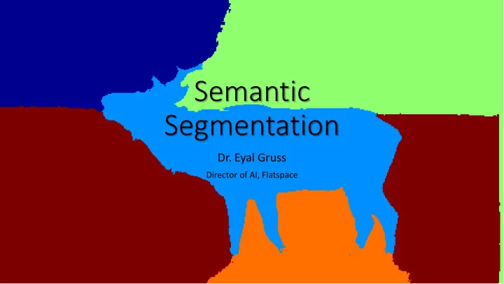
Semantic Segmentation
- Dr. Eyal Gruss
Director of AI, Flatspace
Semantic Segmentation Dr. Eyal Gruss Director of AI, Flatspace - - PowerPoint PPT Presentation
Semantic Segmentation Dr. Eyal Gruss Director of AI, Flatspace Eyal Gruss Talpiyot PhD Physics Machine Learning Researcher Consultant Entrepreneur Digital Artist Flatspace An AI-powered service that creates a VR model from a
Director of AI, Flatspace
Talpiyot PhD Physics Machine Learning
Digital Artist
For photorealistic VR experience
3D Model
Using deep neural networks
Architectural Interpretation Bitmap Floorplan
An AI-powered service that creates a VR model from a simple floorplan.
Demo video: http://flatspace.xyz
28.19% 25.77% 16.42% 11.74% 6.66% 3.57% 2.99% 2.25% 5.10%
0% 5% 10% 15% 20% 25% 30% 2010 2011 2012 2013 2014 2015 2016 2017 Human level Top 5 classification error Move to deep neural networks: AlexNet
GoogLeNet Microsoft Residual Net
1.2M train images, 100k test images, 1000 categories
Trimps- Soushen Ministery
security, China Karpathy Momenta/ Oxford
googleresearch.blogspot.com/2014/09/ building-deeper-understanding-of- images.html (Szegedy et al., GoogLeNet)
Live:
Concurrence, Localization Occlusion Out of context Counting Tracking
Li et al., arxiv.org/abs/1611.07709
Won the COCO 2016 Detection Challenge (for segmentation)
Fischer et al., arxiv.org/abs/1703.01101 Xie et al., arxiv.org/abs/1703.08603 Metzen et al., arxiv.org/abs/1704.05712 Cisse et al., arxiv.org/abs/1707.05373
combine several of the above
aka: scene labeling / scene parsing / dense prediction / dense labeling / pixel-level classification
(d) Input (e) semantic segmentation (f) naive instance segmentation (g) instance segmentation (e) semantic segmentation
Pascal VOC 2012 11,530 6,929 20 + background Train+Validation: github.com/nightrome/really- awesome-semantic-segmentation
background class)
the best
1. Patchwise CNN 2. FCN 3. DeepLab 4. DeconvNet 5. U-Net 6. SegNet 7. Dilated Convolutions (Yu and Koltun) 8. 100-Layer Tiramisu (DesneNets) 9. Wide ResNet 10. PSPNet 11. Adversarial 12. PolygonRNN 13. Mask R-CNN 14. Semi-supervised with unsupervised loss
layers
with a single pass that is much more efficient due to convolution sharing
cs231n_2017_lecture11.pdf
Stride = 2 Stride = 1/2 input
(Resolution Increasing Convolutions)
ImageNet (AlexNet/VGG-16/GoogLeNet) and convert fully connected to conv (conv7)
upsampling to get full spatial output (FCN-32s)
and sum with conv prediction added to pool4
(vs. 50 s)
Before softmax After softmax
hole = atrous = dilated convolutions increase field of view without decreasing resolution,
learned 2x2 upconv + (3x3 regular conv + ReLU) * 2
around morphological edges
use half the filters and padding
dropout
pre-trained on Pascal VOC 2012
ReLUs, with increasing dilations and initialized to unit filters
and trained with fixed front-end
connections
benchmarks
a la DeepLab
+ pyramid pooling module
(2016)
Mismatched Relationship Confusion Categories Inconspicuous Classes
Goodfellow et al., arxiv.org/abs/1406.2661 Generator
תרצוי
Discriminator
(Curator) תרצוא Fake or Real? Fake Real
Isola et al., phillipi.github.io/pix2pix Interactive: affinelayer.com/pixsrv
Guide: ml4a.github.io/guides/Pix2Pix fotogenerator.npocloud.nl
structure)
(ConvLSTM)
arxiv.org/abs/1605.01368
Supervised Proposed 10 pix/image 10 pix/image Full labels GT
learning/pytorch/visdom/2017/06/01/semantic-segmentation-over-the-years