self-consistent field = 1 1 Z X d d r h m ( ~ r ) 2 i = h m 2 i h - PowerPoint PPT Presentation

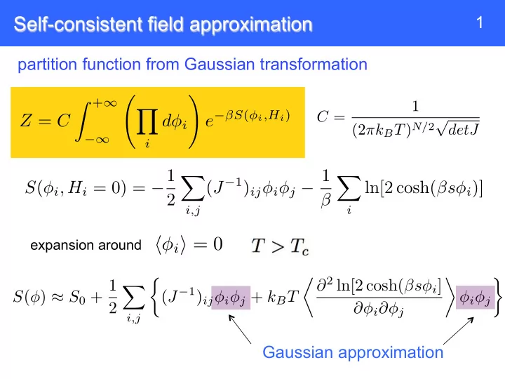
Self-consistent field approximation 1 partition function from Gaussian transformation Z + ∞ Y ! 1 e − β S ( φ i ,H i ) C = Z = C d φ i (2 π k B T ) N/ 2 √ detJ −∞ i S ( φ i , H i = 0) = − 1 ( J − 1 ) ij φ i φ j − 1 X X ln[2 cosh( β s φ i )] 2 β i,j i expansion around h φ i i = 0 ⌧ ∂ 2 ln[2 cosh( β s φ i ] ⇢ � � S ( φ ) ≈ S 0 + 1 X ( J − 1 ) ij φ i φ j + k B T φ i φ j 2 ∂φ i ∂φ j i,j Gaussian approximation

Self-consistent field approximation 2 Gaussian approximation ⇡ S 0 + 1 ⇢ ⌧ 1 �� X ( J − 1 ) ij + β s 2 δ ij S ( φ ) φ i φ j cosh 2 ( β s φ i ) 2 i,j ⇡ S 0 + 1 X � ( J − 1 ) ij + β s 2 δ ij (1 � β 2 s 2 h φ 2 i φ i φ j . 2 i,j uniform φ i = 1 X q e i ~ q · ~ r i Fourier transform: φ ~ h φ 2 i i = h φ 2 i N ~ q ⇢ � = S 0 + 1 1 X q ) + � s 2 (1 � � 2 s 2 h � 2 i ) S ( � ) � ~ q � − ~ q 2 N J ( ~ q ~ a d  q 2 + A + 3 Bs 6 � 3 h � 2 i X � = S 0 + � ~ q � − ~ q 2 J 2 z 2 N ~ q

Self-consistent field approximation 3 = S 0 + a d  q 2 + A + 3 B h m 2 i X � S m ~ q m − ~ q 2 N ~ q φ ~ q = Jzm ~ q = S 0 + 1 X G − 1 ( ~ q ) m ~ q m − ~ q 2 ~ q 0 Z Y � − � G � 1 ( ~ Z 0 = Z 0 dm ~ q dm � ~ q exp q ) m ~ q m � ~ q / 2 ~ q 0 Z 2 + m 00 n o 2 ) / 2 Y − � G � 1 ( ~ dm 0 q dm 00 q )( m 0 = Z 0 q exp ~ ~ ~ ~ q q ~ q 0 Y runs only over a half-space of ~ e.g. { ~ q | q z ≥ 0 } q ~ q

Self-consistent field approximation 4 self-consistent field = 1 1 Z X d d r h m ( ~ r ) 2 i = h m 2 i h m ~ q m � ~ q i L d N 2 q ~ Z 0 0 Z Y � � G � 1 ( ~ � = dm ~ q dm � ~ q m ~ q m � ~ q exp q ) m ~ q m � ~ q / 2 Z 0 L d q ~ self-consistence equation for fluctuations h m 2 i

Self-consistent field approximation - susceptibility 5 susceptibility

Self-consistent field approximation - instabillity 6 instability at cutoff:

Self-consistent field approximation - critical exponents 7 temperature dependence of for cutoff necessary for correlation length

Self-consistent field approximation - critical exponents 8 mean field exponents but Fisher scaling

Self-consistent field approximation - critical exponents 9 regime 1: dominant "close" to regime 2: dominant "far" from mean field