Seiberg-Witten Theory and AGT Relation Tohru Eguchi We consider N = - PowerPoint PPT Presentation

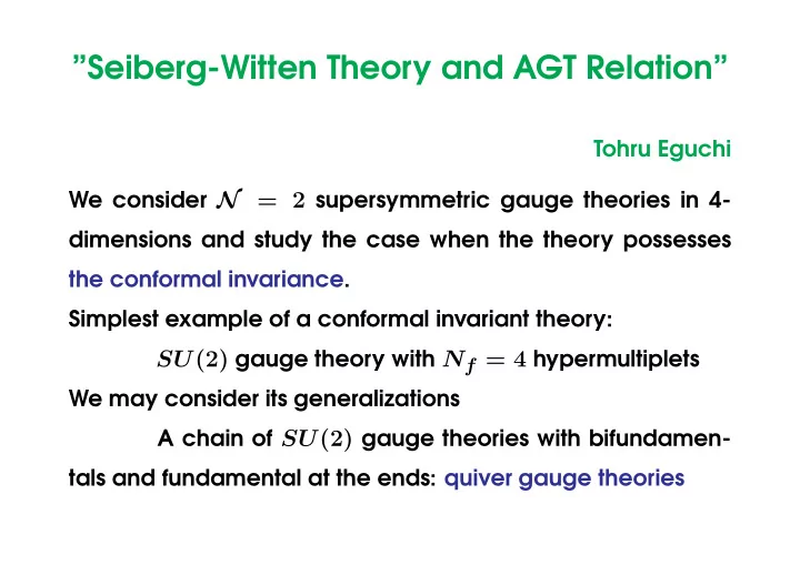
”Seiberg-Witten Theory and AGT Relation” Tohru Eguchi We consider N = 2 supersymmetric gauge theories in 4- dimensions and study the case when the theory possesses the conformal invariance. Simplest example of a conformal invariant theory: SU (2) gauge theory with N f = 4 hypermultiplets We may consider its generalizations A chain of SU (2) gauge theories with bifundamen- tals and fundamental at the ends: quiver gauge theories

As is well-known, such quiver theories are obtained using the brane construction as shown in the figure: One has n + 1 NS5 branes and a pair of D 4 branes are sus-

pended between neighbouring NS5 branes giving rise to SU (2) 1 × SU (2) 2 · · · × SU (2) n gauge symmetry. Two D4 branes at extreme left and right extend to x 6 = ±∞ repre- senting fundamental hypermultiplets. In such a configuration each SU i (2) theory couples to N f = 4 hypermultiplets and is conformally invariant. Thus there exists a set of marginal parameters in the theory π + 8 iπ { τ i = θ i i = 1 , , n } , g 2 i Uplifting this brane configuration to 11 dimensions ⇒ M theory picture with an M5 brane wrapping a Riemann =

surface (cylinder) with punctures. Thus, conformal N = 2 theories ≈ an M5 brane wrapping a Riemann surface C with a number of punctures. Number of parameters of Riemann surface C g,n of genus g

3 g − 3 + n with n punctures: This agrees with the number of gauge theory parameters { τ i } . Hence one expects Gaiotto S-duality group of quiver gauge theory = mapping class group of Riemann surface C g,n

Remarkable observation Alday,Gaiotto,Tachikawa AGT relation ∫ [ da ] | Z Nek ( τ ; a ; m, ϵ i ) | 2 ∏ ⟨ V m i ( τ i ) ⟩ = Liouville Nekrasov partition function of SU (2) gauge theory in Ω background correlation function Liouville momentum external line: m i ∆ i = m i � ( Q − m i  � ) � ,   α = Q 2 + a interbal line:   �

Background charges Q = b + 1 b, c = 1 + 6 Q 2 ϵ 1 = b � , ϵ 2 = � b " # " $ ! " % " &

Nekrasov formula Sum over Yang tableau; Y = ( λ 1 ≥ λ 2 ≥ · · · ) q | ⃗ Y | Z vector ( ⃗ ∑ a, ⃗ a, ⃗ Z Nek = Y ) Z antifund ( ⃗ Y , m 1 ) ( Y 1 ,Y 2 ) a, ⃗ a, ⃗ a, ⃗ × Z antifund ( ⃗ Y , − m 3 ) Z fund ( ⃗ Y , − m 4 ) Y , m 2 ) Z fund ( ⃗

Here ) − 1 ( ∏ ∏ a, ⃗ a ij − ϵ 1 L Y j ( s ) + ϵ 2 ( A Y i ( s ) + 1) Z vector ( ⃗ Y ) = i,j =1 , 2 s ∈ Y i ) − 1 ( ∏ × a ji + ϵ 1 L Y j ( t ) − ϵ 2 ( A Y i ( t ) + 1) + ϵ + t ∈ Y j ∏ ∏ a, ⃗ ( a i + ϵ 1 ( ℓ − 1) + ϵ 2 ( m − 1) − µ + ϵ + ) Z fund ( ⃗ Y , µ ) = i =1 , 2 s ∈ Y i ∏ ∏ a, ⃗ ( a i + ϵ 1 ( ℓ − 1) + ϵ 2 ( m − 1) + µ ) Z antifund ( ⃗ Y , µ ) = i =1 , 2 s ∈ Y i ϵ + = ϵ 1 + ϵ 2 , a ij = a i − a j . L Y ( s ) and A Y ( s ) are leg and arm length of the site s .

Nekrasov formula is obtained by summing over contributions from fixed points in the ADHM formula under gauge and Lorenz transformation ( SO (4) = SU (2) L × SU (2) R ∈ ( ϵ 1 , ϵ 2 ) ). First exact relationship between 4-dim CFT and 2-dim CFT. Higher rank generalization: Toda theories

♠ Attempts at direct proof Fateev-Litvinov Detailed study of the algebraic structure of conformal block in Liouville theory , i.e. the recursion relation by Al.B.Zamolodchikov. R n,m F ∆ m, − n ⟨ V α ⟩ ≈ F ∆ F ∆ ∑ q mn α ( q ) , α ( q ) = ( q ) α ∆ − ∆ m,n and comparison with the sum over Yang tableaus of gauge theory side. Conformal block of 1-point function in Liouville theory on a torus = N = 4 gauge theory perturbed by the mass of the adjoint hypermultiplet ( N = 2 ∗ theory)

♠ Exact Integration Consider Liouville correlation function in free field represen- tation N ∫ e bϕ ( z i ) dz i ⟩ e im a ϕ ( q a ) ∏ ∏ ⟨ a i =1 screening ops. ∫ ∏ ( z i − z j ) − 2 b 2 , ( q a − q b ) 2 m a m b dz i ( z i − q a ) − 2 ibm a ∏ ∏ = a<b i,a i<j ∑ im a + Nb = Q i Dotesnko-Fatteev integral

This is an integration of Selberg type. N N ∫ ( x i − x j ) 2 β ∏ ∏ ∏ x a i (1 − x i ) c I N ( a, c, β ) = dx i i =1 i =1 i<j N − 1 Γ( a + 1 + jβ )Γ( c + 1 + jβ )Γ(1 + ( j + 1) β ) ∏ = Γ( a + c + 2 + ( N + j − 1) β )Γ(1 + β ) j =0 Attempts at exact evaluation and comparison with conformal blocks. Morozov-Kironov-Shakirov, Itoyama-Oota · · ·

♠ Monodromy transformations x 2 = ϕ 2 ( z ) , SW curve Σ : m 2 i ϕ 2 has double poles ≈ ( z − z i ) 2 1 1 1 ∂F � � xdz = a i D , a i xdz = a i , D = 2 πi 2 πi 4 πi ∂a i A i B i In the semi-classical limit � → 0 , ϵ 1 , 2 << a i , m i − F ( a i ) ( ) Z ≈ exp � 2

Liouville stress tensor T ( z ) ⟨ T ( z ) V m 1 ( z 1 ) · · · V m n ( z n ) ⟩ ≈ − 1 � 2 ϕ 2 ( z ) ⟨ V m 1 ( z 1 ) · · · V m n ( z n ) ⟩ ⇓ − m 2 i ∆ i � 2 ( z − z i ) 2 ≈ ( z − z i ) 2 Degenerate field − b 2 ϕ ( z ) which possesses a de- Consider a field Φ 2 , 1 ( z ) = e generacy at level 2 z Φ 2 , 1 ( z ) = − b 2 : T ( z )Φ 2 , 1 ( z ) : ∂ 2

Correlation function with an extra insertion of Φ 2 , 1 Z ( a i ; z ) = ⟨ Φ 2 , 1 ( z ) V m 1 ( z 1 ) · · · V m n ( z n ) ⟩ In the semi-classical limit − F ( a i ) + bW ( a i ; z ) ( ) Z ( a i ; z ) ≈ exp + · · · � 2 � One finds ( ∂W ) 2 = ϕ 2 ( z ) = x ( z ) 2 Hence ∫ z W ± ( z ) = ± z ∗ xdz

shift around A, B cycles gives Z ( a i ; z + A j ) = exp(2 πib a j ) Z ( a i ; z ) � Z ( a i ; z + B j ) = exp(2 πib a j D ) Z ( a i ; z ) � Similarly we may consider the process 1. Insert identity operator inside the Liouville correlator 2. Φ 2 , 1 ⊗ Φ 2 , 1 ≈ 1 3. Transport one of Φ 2 , 1 ’s around A, B cycle 4. Pair annihilate two Φ ’s into identity

⇒ L ( γ ) F α = cos( πb (2 α − Q ) F α = cos( πbQ ) These processes give monodromy factors corresponding to the action of Wilson loop, ’t Hooft loop and surface operators. Alday-Gaiotto-Gukov-Tachikawa-Verlinde Drukker-Gomis-Okuda-Teschner

♠ Matrix Model Dotsenko-Fatteev integral when b = i suggests a matrix model interpretation with an action ∑ m a log( M − q a ) S = a and { z i } are identified as matrix eigenvalues. Dijkgraaf-Vafa We find that this model in fact reproduces Seiberg-Witten the- ory (also for the asymptotically free cases N f = 2 , 3 ). But it still has mysterious features. T.E.-Maruyoshi

Let us consider the simple case of 4 hypermultiplets with masses m ± , ˜ m ± . Define m 0 = 1 2( m + − m − ) , m 1 = 1 m + − ˜ 2( ˜ m − ) m 2 = 1 2( m + + m − ) , m 3 = 1 2( ˜ m + + ˜ m − ) Condition: ∑ m i = 2 g s N i

M theory curve is given by C M : ( v − m + )( v − m − ) z 2 + c 1 ( v 2 + Mv − U ) z + c 1 ( v − ˜ m + )( v − ˜ m − ) = 0 For convenience, set c 1 = − (1 + q ) , c 2 = q . By shifting v to eliminate the linear term and setting v = xz ) 2 m 2 z 2 + (1 + q ) M ( 2 z + m 3 q C M : x 2 = z ( z − 1)( z − q ) 2 ) z 2 − (1 + q ) Uz + ( m 2 +( m 2 0 − m 2 1 − m 2 3 ) q z 2 ( z − 1)( z − q )

Seiberg-Witten differential behaves at a pole as λ SW = xdz m ∗ 2 πi ≈ z − z ∗ Mass appears at residues. Pole at z = 0 , z = ∞ ; residue ± m 1 , ± m 0 . Require pole at z = 1 with residue ± m 2 and z = q with residue ± m 3 = ⇒ M = − 2 q 1 + q ( m 2 + m 3 ) ♣ UV and IR gauge coupling constant

Standard SW curve of N f = 4 in massless case C SW : y 2 = 4 x 3 − g 2 ux 2 − g 3 u 3 Here ( π ) 4 1 ( ϑ 3 ( q ) 8 + ϑ 2 ( q ) 8 + ϑ 4 ( q ) 8 ) g 2 ( ω 1 , q ) = , 24 ω 1 ( π ) 6 1 ϑ 4 ( q ) 4 − ϑ 2 ( q ) 4 ) ( g 3 ( ω 1 , q ) = ω 1 432 ( 2 ϑ 3 ( q ) 8 + ϑ 4 ( q ) 4 ϑ 2 ( q ) 4 ) × On the other hand M theory curve in the masssless limit is

given by (1 + q ) U C M : x 2 = − z ( z − 1)( z − q ′ ) Here U is related to u = trϕ 2 as U = Au and we have used q ′ in order to distinguish it from q of C SW . By comparing the periods we find q ′ = ϑ 2 ( q ) 4 1 ϑ 3 ( q ) 4 , A = ϑ 2 ( q ) 4 + ϑ 3 ( q ) 4

We regard q in SW curve as the gauge coupling in the infra- red regime q = q IR and q ′ in M theory curve as the ultra- violet gauge coupling constant q ′ = q UV . Relation q UV = ϑ 2 ( q IR ) 4 ϑ 3 ( q IR ) 4 has been obtained by various authors. Grimm et al, Marshakov et al ♠ Matrix model and modular invariance Equation of motion 1 m i ∑ ∑ + 2 g s = 0 λ I − q i λ I − λ J I ̸ = J

We have q 1 = 0 , q 2 = 1 , q 3 = q UV . Eigenvalue distribution is as given in the figure.

Resolvent of the theory is defined by 1 R m ( z ) = g s T r z − M and satisfies the loop equation ⟨ R m ( z ) ⟩ 2 = −⟨ R m ( z ) ⟩ W ′ ( z ) + f ( z ) 4 3 ⟨ ⟩ W ′ ( z ) − W ′ ( M ) c i ∑ f ( z ) = 4 g s T r = z − M z − q i i =1 Matrix model curve (spectral curve) is defined by the dis-

criminant of the loop eq. C spec.curve : x 2 = W ′ ( z ) 2 + f ( z ) ) 2 + ( m 2 i m 2 0 − ∑ i ) z + qc 1 ( m 1 m 2 m 3 = + z − 1 + z − q z ( z − 1)( z − q ) z ∑ ⇒ Eq. of motion = c i = 0 i ⇒ c 2 + qc 3 = m 2 m i ) 2 ∑ Residue at ∞ being ± m 0 = 0 − ( Then qc 1 = (1 + q ) m 2 1 + (1 − q ) m 2 3 + 2 qm 1 m 2 − 2 qm 2 m 3 +2 m 1 m 3 − (1 + q ) U ⇒ C W = C spec.curve =