Scientific Data Compression: From Stone-Age to Renaissance Factor - - PowerPoint PPT Presentation

scientific data compression from stone age to renaissance
SMART_READER_LITE
LIVE PREVIEW

Scientific Data Compression: From Stone-Age to Renaissance Factor - - PowerPoint PPT Presentation

Scientific Data Compression: From Stone-Age to Renaissance Factor 10,100 compression Background Focus on spatial compression Best in class lossy compressor Point wise max error bound: 10 -5 Open questions Random noise


slide-1
SLIDE 1

Scientific Data Compression: From Stone-Age to Renaissance

Franck Cappello

Argonne National Lab and UIUC CCDSC, October 2016

  • Background
  • Focus on spatial compression
  • Best in class lossy compressor
  • Open questions

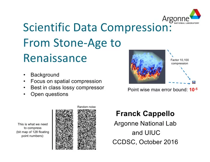
This is what we need to compress (bit map of 128 floating point numbers):

Random noise Factor 10,100 compression

Point wise max error bound: 10-5

slide-2
SLIDE 2

Why compression?

— Today’s scientific research is using simulation or

instruments and produces extremely large of data sets to process/analyze

— In some cases, extreme

data reduction is needed:

— Cosmology Simulation (HACC):

— A total of >20PB of data when

simulating trillion of particles

— Petascale systems FS ~20PB

(you will never have 20PB of scratch for one application)

— On Blue Waters (1TB/s file system), it would take

20 X 10^15 / 10^12 seconds (5h30) to store the data

à currently drop 9 snapshots over 10

— Also: HACC uses all the available memory: there is room only

for 1 snapshot (so temporal compression would not work)

slide-3
SLIDE 3

Stone age of compression for scientific data sets

— Tools were rudimentary

à Apply compressors developed for integer strings (GZIP, BZIP2) or images (JPEG2000)

— Tool effects were limited in power and precision

à Low compression factors à First lossy compressors did not control errors

— No clear understanding on how to improve technology

à Some did not understand the limits of Shannon entropy à Metrics were rudimentary: compression factor & speed

— Cultural fear of using lossy compression for data reduction

10 years ago

slide-4
SLIDE 4

Artefacts of that period (lossless)

— LZ77: leverages repetition of symbol string — Variable Length Coding (Huffman for example) — Move to front encoding — Arithmetic encoding (symbols are

segments of a line [0,1] of length proportional to their probability of

  • ccurrence)

— Burrows–Wheeler algorithm (bzip2) — Markov Chain Compression — Dynamic Statistical Encoding (adapts dynamically the probability

table of symbols for Variable Length Coding)

— Lorenzo predictor + correction — Techniques are combined in most powerful compressors: bzip:

Burrows–Wheeler + Move to front + Huffman All these algorithms either leverage string of symbols (bytes) repetition OR perform probability encoding: variable length coding

slide-5
SLIDE 5

Effectiveness of the tools from that period

  • P. Ratanaworabhan, Jian Ke ; M. Burtscher Cornell Univ., Ithaca, NY, USA

Fast lossless compression of scientific floating-point data Data Compression Conference (DCC'06) 2006

Compression limited to a factor of 2 in most cases

In SPPM data set, each double value is repeated ~10 times

slide-6
SLIDE 6
  • 0.00015
  • 0.0001
  • 5e-05

5e-05 0.0001 1000 1500 2000 2500 300 Data Value Linearized Index

0.0001 0.00012 0.00014 0.00016 0.00018 0.0002 1 2 3 4 5 6 7 Data Value Linearized Index 10.6 10.65 10.7 10.75 10.8 500 1000 1500 2000 2500 3000 3500 Data Value Linearized Index

  • 2e-05
  • 1.5e-05
  • 1e-05
  • 5e-06

5e-06 1e-05 1.5e-05 2e-05 10000 10200 10400 10600 10800 110 Data Value Linearized Index

APS mouse brain

CESM/ ACME

OCEAN ATM

Reference height humidity

ATM

Total grid-box cloud ice water path Flux of Heat in grid-y direction

Renaissance: the current period (1)

Scientific dataset need specific compressors.. …exploiting their unique properties.

But not all datasets are smooth

0.02 0.04 0.06 0.08 0.1 0.12 0.14 0.16 0.18 1000 2000 3000 4000 5000 6000 7000 8000 900 Data Value Linearized Index 700 800 900 1000 1100 1200 1300 1400 2000 4000 6000 8000 100 Data Value Linearized Index

FLASH (Sedov) Hurricane Plotting datasets as time series:

slide-7
SLIDE 7

Renaissance (2): Increased acceptance of lossy compression

— Tradeoff between data size and data accuracy — Specific requirements for usefulness:

— Error-bounded compression: guaranteeing the accuracy of the

decompressed data for users (multiple metrics). à Max error: Typically 10-5, à PSNR (f(dynamic, mean squared error)) =>100DB (105)

— Fast compression and decompression (if in-situ, compression time

should not exceed significantly storage time): x100MB/s on 1 core

Compression Decompression Compressed data

1/100 of initial size

Data Data + e

slide-8
SLIDE 8

Renaissance (3): Explosion

  • f new ideas

— Lossy compressors

— ANL/SZ, FPZIP-40, ZFP, ISABELA, SSEM, NUMARCK.

— Common techniques used by related work

— Vector Quantization (VQ), Transforms (T), Curve-Fitting/Spline

interpolation (CFA), Binary Analysis (BA), Lossless compress (Gzip), Sorting (only Isabella), Delta encoding (only NUMARCK), Lorenzo predictor (only FPZIP)

slide-9
SLIDE 9

Argonne SZ Best in class compressor for scientific

data sets (strictly respecting user set error bounds).

— Basic Idea of SZ 1.1 (four steps):

Step 1. Data linearization: Convert N-D data to 1-D sequence Step 2. Approximate/Predict each data point by the best-fit curve- fitting models Step 3. Compress unpredictable data by binary analysis Step 4. Perform lossless compression (Gzip): LZ77, Huffman coding Steps 1-3 prepare for strong Gzip compression

…...

i i-1 i+1 i+2 i-2 … … Data index Data values

slide-10
SLIDE 10

Step 2 of SZ 1.1: Prediction

by best-fit curve fitting model

— Use two-bit code to denote the best-fit curve-fitting model — 01: Preceding Neighbor Fitting (PNF) — 10: Linear Curve Fitting (LCF) — 11: Quadratic Curve Fitting (QCF) — 00: This value cannot be predicted – unpredictable data

Predicted Value Decompressed Value 1-D array data value i-1 i i-2 i-3 Quadratic Curve Fitting Linear Curve Fitting Preceding Neighbor Fitting

user-required error bound

Original Data Value Xi

(L)

Xi

(N)

Xi

(Q)

slide-11
SLIDE 11

SZ 1.1 Error control

— Two types of error bounds are supported

— Absolute Error Bound Specify the max compression error by a constant, such as 10-6 — Relative Error Bound Specify the max compression error based on the global value range size and a percentage

Combination of Error Bounds

Users can set the real compression error bound based on only absErrorBound, relBoundRatio, or a kind of combination of them. Two types of combinations are provided: AND, OR. The combined error bound is then computed by the Min of the two error bounds (AND) or the Max (OR)

slide-12
SLIDE 12

Evaluation Results

— Compression Factor (EB: 10-6): original size / compressed

size

— SZ 1.1 Compression Factor > 10 for 7 of the 13 benchmarks — SZ 1.1 better than ZFP for all datasets but 2

1.1

slide-13
SLIDE 13

Evaluation Results

— Compression Error

— Cumulative Distribution Function over the snapshots — SZ and ZFP can both respect the absolute error bound 10-6 well. — SZ is much closer to the error bound (ZFP over preserves data

accuracy)

SZ ZFP

However, in some situations ZFP does not respect the error bound (observed on the ATM dataset from NCAR)

slide-14
SLIDE 14

Evaluation Results

— Compression Time (in seconds)

ATM 1.5TB - 25604 24121 38680 Hurricane 4.8GB 1152 155 156 237 High cost due to sorting operations SZ 1.1 compression time is comparable to ZFP

slide-15
SLIDE 15

More research is needed (1)

Some datasets are “hard to compress”

— All compressors (including SZ) fail to reach high

compression factors on several data sets:

— BlastBS (3.65), CICE (5.43), ATM (3.95), Hurricane (1.63) — We call these data sets “hard to compress”

— A common feature of these datasets is the presence

  • f spikes

— If you plot the dataset as a time series:

— Example: — APS data

(Argonne photon source)

slide-16
SLIDE 16

More research is needed (2):

What are the right metrics?

Uncompressed Compressed (10-4) Compression rate (bits/value)

0.0001 0.001 0.01 0.1 1 1/N 6/N 11/N 16/N 21/N 26/N 31/N 36/N 41/N 46/N Amplitude Frequency

Spectral density estimation

0.0001 0.001 0.01 0.1 1 1/N 6/N 11/N 16/N 21/N 26/N 31/N 36/N 41/N 46/N Amplitude Frequency

Spectral density estimation

0.002 0.004 0.006 0.008 0.01 1 6 11 16 21 26 31 36 41 46 Correlation Coefficient Distance Delta

Autocorrelation of Compression Error

0.009 0.0094 0.0098 0.0102 0.0106 0.011 Frequency Decompressed Error

Distribution of Decompression Error

20 40 60 80 100 120 140 160 5 10 15 20 25 PSNR (dB) Rate (bits/value)

Rate-Distortion

SZ Compression factor: 6.4 (1.4 with GZIP)

Uniform white noise Compression adds extra correlation

Variable FREQSH (Fractional occurrence of shallow convection) in ATM Data Sets (CESM/CAM)

Laplacian comparison

(original versus compressed)

slide-17
SLIDE 17

More research is needed (3):

Respecting error bound does not guarantee temporal behavior

SZ1.1 SZ1.3

  • PlasComCM: coupled multi-physics plasma combustion code (UIUC) solving

compressible Navier-Stokes equations.

  • Truncation error is at 10-5
  • We checkpoint it and restart from lossy (EB=10-5) checkpoints.
  • We measure derivation from lossless restarts
  • Two different algorithms SZ 1.1 (CF:~5) and SZ 1.3 (CF:~6)

Gaz Cylinder

(Images: Jon Calhoun, UIUC)

slide-18
SLIDE 18

More research is needed (4):

Respecting error bound does not guarantee spatial behavior

SZ1.1 SZ1.3

Maximal absolute error between the numerical solution of momentum and the compressed numerical solution of momentum in PlasComCM.

(Images: Jon Calhoun, UIUC)

slide-19
SLIDE 19

Conclusion

— The world of compression is fascinating!

— This is just the beginning.

— There is still a lot to be done:

— ”Hard to compress data sets” — Identify relevant compression metrics — Understand/control propagation of

compression error

— Opportunities for co-design

— Preparing a workshop at Argonne in

March 2017 ”Lossy compression for scientific computing and data analytics”

— If you interested, send me an email.

By the way, compression is also an art