Scatterplot of y versus x Regression Line Superimposed Residual - - PDF document

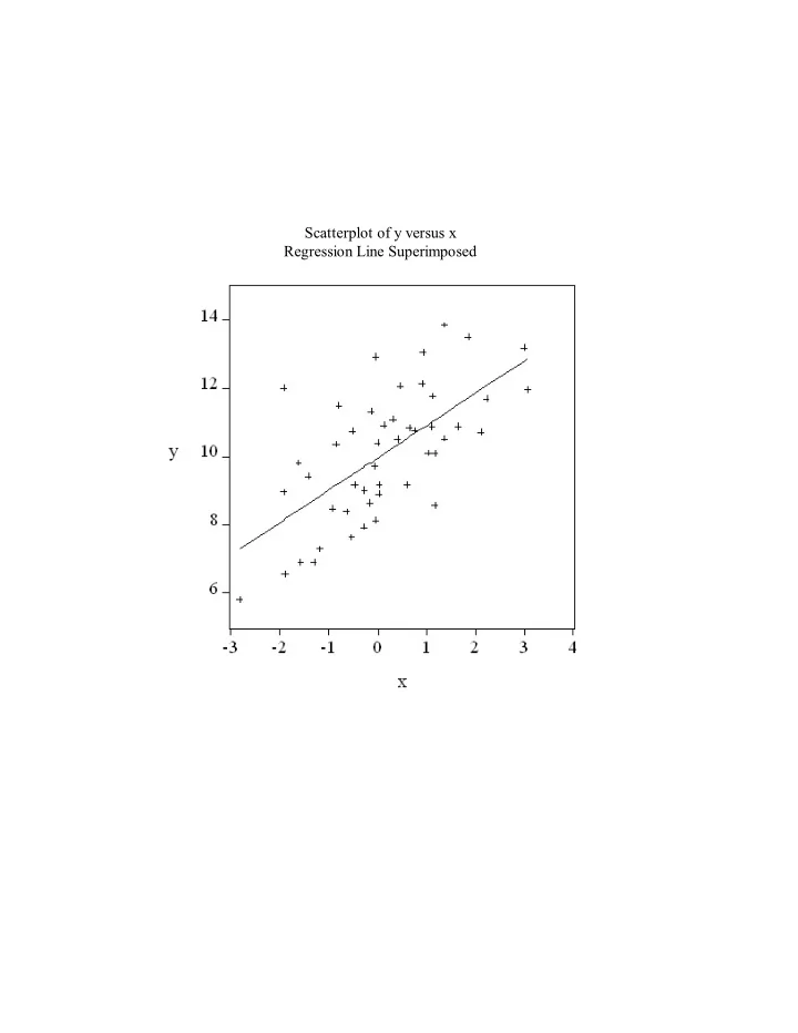
Scatterplot of y versus x Regression Line Superimposed

Residual Plot Regression of y on x and z

1-Year Treasury Bond Rate

Change in 1-Year Treasury Bond Rate

Liquor Sales

Histogram and Descriptive Statistics Change in 1-Year Treasury Bond Rate

Scatterplot 1-Year versus 10-Year Treasury Bond Rate

Scatterplot Matrix 1-, 10-, 20-, and 30-Year Treasury Bond Rates

Modeling and Forecasting Trend

• 1. Modeling Trend

Labor Force Participation Rate Females

Labor Force Participation Rate Males

Increasing and Decreasing Linear Trends

Linear Trend Female Labor Force Participation Rate

Linear Trend Male Labor Force Participation Rate

Volume on the New York Stock Exchange

Various Shapes of Quadratic Trends

Quadratic Trend Volume on the New York Stock Exchange

Log Volume on the New York Stock Exchange

Various Shapes of Exponential Trends

Linear Trend Log Volume on the New York Stock Exchange

Exponential Trend Volume on the New York Stock Exchange

Selecting Models

Consistency Efficiency

Degrees-of-Freedom Penalties Various Model Selection Criteria

Retail Sales

Retail Sales Linear Trend Regression Dependent Variable is RTRR Sample: 1955:01 1993:12 Included observations: 468 Variable Coefficient

• Std. Error

T-Statistic Prob. C

• 16391.25

1469.177

• 11.15676

0.0000 TIME 349.7731 5.428670 64.43073 0.0000 R-squared 0.899076 Mean dependent var 65630.56 Adjusted R-squared 0.898859 S.D. dependent var 49889.26 S.E. of regression 15866.12 Akaike info criterion 19.34815 Sum squared resid 1.17E+11 Schwarz criterion 19.36587 Log likelihood

• 5189.529

F-statistic 4151.319 Durbin-Watson stat 0.004682 Prob(F-statistic) 0.000000

Retail Sales Linear Trend Residual Plot

Retail Sales Quadratic Trend Regression Dependent Variable is RTRR Sample: 1955:01 1993:12 Included observations: 468 Variable Coefficient

• Std. Error

T-Statistic Prob. C 18708.70 379.9566 49.23905 0.0000 TIME

• 98.31130

3.741388

• 26.27669

0.0000 TIME2 0.955404 0.007725 123.6754 0.0000 R-squared 0.997022 Mean dependent var 65630.56 Adjusted R-squared 0.997010 S.D. dependent var 49889.26 S.E. of regression 2728.205 Akaike info criterion 15.82919 Sum squared resid 3.46E+09 Schwarz criterion 15.85578 Log likelihood

• 4365.093

F-statistic 77848.80 Durbin-Watson stat 0.151089 Prob(F-statistic) 0.000000

Retail Sales Quadratic Trend Residual Plot

Retail Sales Log Linear Trend Regression Dependent Variable is LRTRR Sample: 1955:01 1993:12 Included observations: 468 Variable Coefficient

• Std. Error

T-Statistic Prob. C 9.389975 0.008508 1103.684 0.0000 TIME 0.005931 3.14E-05 188.6541 0.0000 R-squared 0.987076 Mean dependent var 10.78072 Adjusted R-squared 0.987048 S.D. dependent var 0.807325 S.E. of regression 0.091879 Akaike info criterion

• 4.770302

Sum squared resid 3.933853 Schwarz criterion

• 4.752573

Log likelihood 454.1874 F-statistic 35590.36 Durbin-Watson stat 0.019949 Prob(F-statistic) 0.000000

Retail Sales Log Linear Trend Residual Plot

Retail Sales Exponential Trend Regression Dependent Variable is RTRR Sample: 1955:01 1993:12 Included observations: 468 Convergence achieved after 1 iterations RTRR=C(1)*EXP(C(2)*TIME) Coefficient

• Std. Error

T-Statistic Prob. C(1) 11967.80 177.9598 67.25003 0.0000 C(2) 0.005944 3.77E-05 157.7469 0.0000 R-squared 0.988796 Mean dependent var 65630.56 Adjusted R-squared 0.988772 S.D. dependent var 49889.26 S.E. of regression 5286.406 Akaike info criterion 17.15005 Sum squared resid 1.30E+10 Schwarz criterion 17.16778 Log likelihood

• 4675.175

F-statistic 41126.02 Durbin-Watson stat 0.040527 Prob(F-statistic) 0.000000

Retail Sales Exponential Trend Residual Plot

Model Selection Criteria Linear, Quadratic and Exponential Trend Models Linear Trend Quadratic Trend Exponential Trend AIC 19.35 15.83 17.15 SIC 19.37 15.86 17.17

• 3. Forecasting Trend

Retail Sales History, 1990.01 - 1993.12 Quadratic Trend Forecast, 1994.01-1994.12

Retail Sales History, 1990.01 - 1993.12 Quadratic Trend Forecast and Realization, 1994.01-1994.12

Retail Sales History, 1990.01 - 1993.12 Linear Trend Forecast, 1994.01-1994.12

Retail Sales History, 1990.01 - 1993.12 Linear Trend Forecast and Realization, 1994.01-1994.12

Modeling and Forecasting Seasonality

• 1. The Nature and Sources of Seasonality
• 2. Modeling Seasonality

1

D = (1, 0, 0, 0, 1, 0, 0, 0, 1, 0, 0, 0, ...)

2

D = (0, 1, 0, 0, 0, 1, 0, 0, 0, 1, 0, 0, ...)

3

D = (0, 0, 1, 0, 0, 0, 1, 0, 0, 0, 1, 0, ...)

4

D = (0, 0, 0, 1, 0, 0, 0, 1, 0, 0, 0, 1, ...)

Gasoline Sales

Liquor Sales

Durable Goods Sales

Housing Starts, 1946.01 - 1994.11

Housing Starts, 1990.01 - 1994.11

Regression Results Seasonal Dummy Variable Model Housing Starts LS // Dependent Variable is STARTS Sample: 1946:01 1993:12 Included observations: 576 Variable Coefficient

• Std. Error

t-Statistic Prob. D1 86.50417 4.029055 21.47009 0.0000 D2 89.50417 4.029055 22.21468 0.0000 D3 122.8833 4.029055 30.49929 0.0000 D4 142.1687 4.029055 35.28588 0.0000 D5 147.5000 4.029055 36.60908 0.0000 D6 145.9979 4.029055 36.23627 0.0000 D7 139.1125 4.029055 34.52733 0.0000 D8 138.4167 4.029055 34.35462 0.0000 D9 130.5625 4.029055 32.40524 0.0000 D10 134.0917 4.029055 33.28117 0.0000 D11 111.8333 4.029055 27.75671 0.0000 D12 92.15833 4.029055 22.87344 0.0000 R-squared 0.383780 Mean dependent var 123.3944 Adjusted R-squared 0.371762 S.D. dependent var 35.21775 S.E. of regression 27.91411 Akaike info criterion 6.678878 Sum squared resid 439467.5 Schwarz criterion 6.769630 Log likelihood

• 2728.825

F-statistic 31.93250 Durbin-Watson stat 0.154140 Prob(F-statistic) 0.000000

Residual Plot

Estimated Seasonal Factors Housing Starts

• 3. Forecasting Seasonal Series

Housing Starts History, 1990.01-1993.12 Forecast, 1994.01-1994.11

Housing Starts History, 1990.01-1993.12 Forecast and Realization, 1994.01-1994.11