SAR Phenomenology Dr. Armin Doerry Detailed contact information at - PDF document

10/12/2017 SAR Phenomenology Dr. Armin Doerry Detailed contact information at www.doerry.us This presentation is an informal communication intended for a limited audience comprised of attendees to the Institute for Computational and Experimental Research in Mathematics (ICERM) Semester Program on "Mathematical and Computational Challenges in Radar and Seismic Reconstruction“ (September 6 ‐ December 8, 2017). 1 This presentation is not intended for further distribution, dissemination, or publication, either whole or in part. 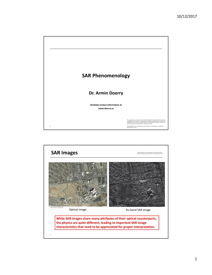SAR Images All SAR images in this presentation are Courtesy of Sandia National Laboratories, Airborne ISR, unless otherwise noted. Image courtesy of Google Earth Optical image Ku‐band SAR image While SAR images share many attributes of their optical counterparts, the physics are quite different, leading to important SAR image characteristics that need to be appreciated for proper interpretation. 2 1

10/12/2017 Image Basics – Pixel Spacing Pixel – Pixels are “picture elements” that make up an image. – their ‘spacing’ is not necessarily the image resolution. • the ratio of resolution to pixel spacing is the ‘oversampling factor’ – We generally desire pixel spacing to be finer than the resolution – typically 1.18 to 1.5 for many SAR systems. same resolution, but coarser pixel spacing Image Basics – Resolution 1.0 m resolution 0.3 m resolution 0.1 m resolution Finer resolution clearly offers more detail – but at the expense of greater latency and more complicated processing 4 2

10/12/2017 Geometric Distortions ‐ Layover Sphere of Cone of constant constant range Doppler * * Ground plane The intersection of constant range and constant Doppler manifests as a circle. All locations on the circle have same range and Doppler. This circle intersects the ground at as many as two locations. The real antenna beam selects which of these makes it into the data. However, any target above or below the ground on the circle and in the beam will map to the ground intersection point. This is called “layover.” 5 Geometric Distortions – Layover Far range constant range contour Since the SAR renders range, tops of tall objects are nearer to the radar than their bottoms, so appear at nearer ranges in the SAR image. They ‘lean forward’ towards the radar, projecting to nearer ranges. This is the opposite of optical images, which causes tops of tall objects to lean away, projecting to farther ranges on the ground. Near range 6 3

10/12/2017 Geometric Distortions – Layover Near range By rotating the image so that near range is at the top of the image, the image looks more natural. This is more a matter of personal preference. ground plane Far range 7 Geometric Distortions – Layover Shadow Layover Layover is in the direction towards the Layover is in the direction towards the closest approach of the flight path. closest approach of the flight path. Shadows are always away from the Shadows are always away from the radar. radar. Consequently shadows are not always Consequently shadows are not always opposite the layover direction. opposite the layover direction. 8 4

10/12/2017 Geometric Distortions The “Ground plane” is a locally level plane at the SRP. The “Slant Plane” customarily Slant plane refers to the plane defined by the radar’s straight‐line flight path and the SRP. Ground plane SRP Literature often refers to “Slant‐plane images” versus “Ground‐plane images.” In both cases the image is still of the ground, and focused to the ground. The distinction often refers to pixelation of the image, and whether it is in equal increments of slant range, or equal increments of ground‐range. Layover is, of course, unaffected. 9 Geometric Distortions – Range‐Doppler Grid Constant‐range spheres intersect the ground as circles, and constant‐Doppler cones intersect the ground as hyperbolas. Consequently, a range‐Doppler grid is ‘warped’ with respect to a Cartesian grid on the ground. 10 8 This manifests most evident with ‘wide‐ 6 angle’ SAR images, especially at finer 4 resolutions and nearer ranges. 2 y For small areas significantly 0 far away in a broadside direction, -2 the local range‐Doppler grid is -4 approximately square. -6 -8 -10 -10 -5 0 5 10 x 10 5

10/12/2017 Imaging Geometry slant range vs. ground range – consider two targets that are not too far apart in range – difference in slant range will be less than difference in ground range • related by the cosine of the local grazing angle     cos r y g   cos grazing angle g (nearly same for both targets) – also true for resolution • most accurate if using the actual depression angle to the target     cos • using nominal depression angle at SRP often r y g a good approximation 11 Imaging Geometry The actual grazing angle changes slightly over the imaged swath. • shallower at farther ranges, • steeper at nearer ranges. – more noticeable as swath width becomes an increasing fraction of the slant range. 12 6

10/12/2017 Imaging Geometry Equal ground spacing does not appear as equal slant‐ range spacing. – appear farther apart at far ranges, – appear closer together at near ranges. This is the native output for range‐Doppler image formation algorithms like the Polar Format Algorithm (PFA). Of course images can always be resampled to other grids. This is not an issue for SAR image with equal tomographic algorithms slant‐range spacing like Backprojection ground truth effect is in range only, not azimuth (other effects in azimuth) 13 Geometric Distortions – Range‐Doppler Grid Note “curve” in roads UHF 14 7

10/12/2017 Canonical Reflectors Canonical reflectors are those for which the RCS is simple and can be calculated in closed‐form solution. They are generally intended to approximate a singular point reflector which is particularly useful for evaluating the ‘goodness’ of SAR images. 15 Canonical Reflectors Canonical reflector arrays are often used as SAR system test sites, to gauge performance of the SAR system during flight. 16 8

10/12/2017 Target Scattering – A sphere (e.g. domed/rounded surfaces) • isotropic – looks the same from any direction • RCS depends on radii of curvature • looks like a point target or a blob – Cylinder (e.g. pipelines, utility wires, weak structural edges, fences) • single‐axis isotropic – RCS peak broadside to cylinder • RCS proportional to diameter strong • looks like a line 17 Target Scattering – Flat Plate (e.g. lake, roads, runways, paved areas) strong • not isotropic at all weak – narrow RCS peak when normal to surface – like a mirror • looks like a point or blob at normal incidence • looks dark at non‐normal incidence – Dihedrals (e.g. buildings, stationary vehicles) • nearly single‐axis isotropic – within inside envelope – RCS peak normal to dihedral joining edge • RCS proportional to plate sizes • looks like a line – located at joining edge 18 9

10/12/2017 Target Scattering – Top Hat (e.g. utility poles, tree trunks, vent pipes) • nearly isotropic • RCS depends on dimensions • looks like a point target or blob – Trihedrals (corner reflectors) (e.g. building inside corners, window wells, truck beds) • nearly isotropic – within inside envelope • RCS proportional to plate sizes • looks like a point or blob – located at apex 19 Complicated Targets Even just a handful of 90 40 RCS (dBsm) scatterers within a 120 60 scatterer position resolution cell will 30 interfere with each other 20 150 30 (adding in and out of phase) so that the RCS is 10 a complicated and sensitive function of 180 0 aspect angle. This is the basis for Swerling models; 210 330 statistical models of RCS depending on nature of scatterers and whether 240 300 they remain coherent 270 from pulse‐to‐pulse, or scan‐to‐scan. 20 10

10/12/2017 Slicy An interesting ‘quasi’‐standard target for a number of SAR target recognition studies is known as “Slicy”, which is made up of a special arrangement of cutouts and other canonical components. 21 Distributed Clutter – Speckle The “graininess” in a SAR The “graininess” in a SAR image is due to the distributed image is due to the distributed nature of the target area, and nature of the target area, and the fact that the waveform is the fact that the waveform is coherent and relatively coherent and relatively narrow‐band. narrow‐band. The patch of ground that is The patch of ground that is contained in a resolution cell is contained in a resolution cell is in fact a complicated scatterer, in fact a complicated scatterer, with RCS that depends on the with RCS that depends on the superposition of many tiny superposition of many tiny surface elements. surface elements. Consequently, the RCS is Consequently, the RCS is generally described generally described statistically per unit area. statistically per unit area. Ku‐band 22 11