Review: Perceptual issues in Graphics Review: lectures 22, 23 - PowerPoint PPT Presentation

Review: Perceptual issues in Graphics Review: lectures 22, 23 lecture 25 In many computer graphics techniques, we can get away with We have discussed several physical aspects of displays. approximations without people noticing. This allows us to save space and/or time. image displays - color - display can be either a projector or a monitor Examples: - spectrum of emitted light at each pixel is a weighted sum of RGB spectra - level of detail (meshes lecture 11) - Weber/Fechner/Stevens Laws - trichromacy and metamerism - anaglyph: 3D stereo displays - shading (if X is smooth, then we can sample & interpolate) - gamma encoding - dynamic range - environment mapping - gamma correction (we are not able to judge the correctness of mirror reflections) - high dynamic range (HDR) scenes and images, - display calibration - tone mapping and low dynamic range (LDR) displays How can one quantify the differences that people can detect - limitations of 'global tone mapping operators' (eye candy) Today, we will concentrate on the latter. ? Intensity Discrimination Example: Intensity Discrimination "Just Noticable Difference" (JND) (a general problem in human perception) - taste: In the figure below, is the center is slightly brighter or darker than n vs n + n grams of sugar per 100 ml - taste: the surround ? - sweetness (# ml of sugar dissolved into water), - hearing (dB) Seems trivial. But when the center intensity is very close to the - saltiness, spicyness, etc. n vs. n + n loudness units (unspecified) surround intensity, the center will not be visible. n vs. n + n Hz (cycles per second of tone) - hearing (dB) The question is, how small a difference can you notice? loudness, frequency - touch (weight) - n vs. n + n Newtons The answer to this question is called the JND. - touch - pressure, weight - vision - brightness - vision - hue - brightness - saturation - hue - saturation JNDs are typically non-linear functions of the intensity. 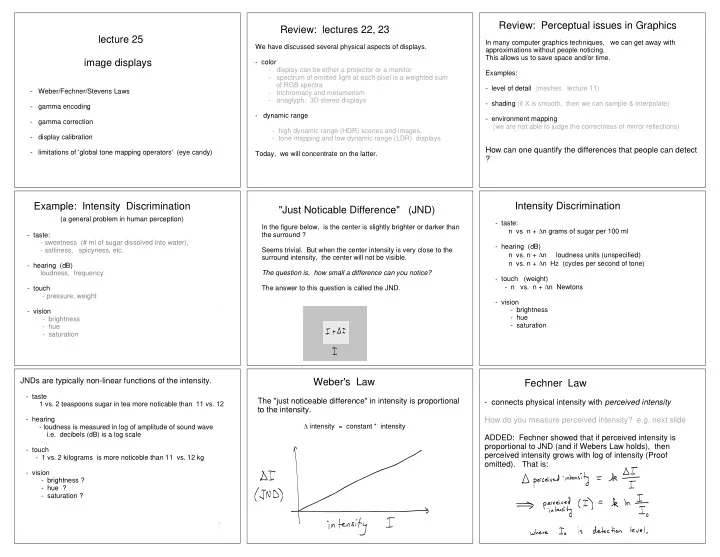Weber's Law Fechner Law - taste The "just noticeable difference" in intensity is proportional - connects physical intensity with perceived intensity 1 vs. 2 teaspoons sugar in tea more noticable than 11 vs. 12 to the intensity. - hearing How do you measure perceived intensity? e.g. next slide intensity = constant * intensity - loudness is measured in log of amplitude of sound wave i.e. decibels (dB) is a log scale ADDED: Fechner showed that if perceived intensity is proportional to JND (and if Webers Law holds), then - touch perceived intensity grows with log of intensity (Proof - 1 vs. 2 kilograms is more noticeble than 11 vs. 12 kg omitted). That is: - vision - brightness ? - hue ? - saturation ?

Steven's Law Example: intensity of light From Fechner's law, we would expect perceived intensity to grow with log of physical intensity. Choose N=10 neutral (R = G = B) values of intensity such that they appear uniformly spaced, or equally discriminable. Such an experiment allows us to connect perceived intensity with physical intensity. appeared in Science 1961 http://sonify.psych.gatech.edu/~walkerb/classes/perception/readings/Stevens1961.pdf Recall last lecture: lecture 25 Camera Response & "compressive non-linearity" One standard model for vision is that perceived intensity ("brightness") is related to physical intensity by image displays approximately a power law. This is consistent with Steven's Law. - Weber/Fechner/Stevens Laws http://en.wikipedia.org/wiki/Lab_color_space - gamma encoding - gamma correction - display calibration - limitations of 'global tone mapping operators' (eye candy) exposure, E * t We are more sensitive to changes in physical intensity at small values of intensity. i.e. the JND's are smaller at This compressive non-linearity is consistent with the laws of Weber/ small intensity values. (True for Weber/Fechner too.) Fechner/Stevens. The encoding of physical intensity is more precise at small intensities than at large intensities. What does gamma encoding achieve? Gamma Encoding (power law) The displayed image on the previous slide does not reproduce the original dynamic range in the scene. Why not? Because we are using Consider a scene such that part of it is in shadow and part is in direct sunlight, a low dynamic range display to show this image! such as the one below. If you were in the real scene (which has very high dynamic range i.e. HDR), you would be able to discriminate small intensity Film cameras: So what are the intensities actually being displayed here ? differences within the shadow region (because of Weber/Fechner/Stevens laws). I will get to that in the rest of the lecture. Until 2005, most cameras used film. The film response function was a compressive non-linearity, namely the opacity of the film varied as a The image below shows a log mapping of the HDR intensities. It enables us to power law with the exposure. The exponent was typically called discriminate the intensities in the darker parts of the scene. but we will say 1/ to be consistent with how we use later. Recall this example from Digital cameras (two step encoding): last lecture: The image was obtained First, encode with linear response, 12 bits per RGB channel (RAW). by computing a HDR image from a set of Second, convert from RAW to JPEG or TIFF, 8 bits per RGB value. JPGs, and then re- JPEG and TIFF use a compresive non-linearity, namely a power law with mapping the intensities an exponent 1/ = 1 / 2.2. We refer to it as "gamma encoding". using a compressive non-linearity (log). http://www.cambridgeincolour.com/tutorials/gamma-correction.htm

The gamma expansion cancels the gamma compression, if one is Gamma expansion (display) lecture 25 indeed exactly the inverse of the other. (In practice, the two models are only approximately gamma power laws, so they don't exactly cancel). image displays eye - Weber/Fechner/Stevens Laws pixel physical intensity linear encoding gamma encoding gamma expansion values - gamma encoding - gamma correction monitor - display calibration - limitations of 'global tone mapping operators' (eye candy) Most monitors and projectors emit an RGB intensity (to be more precise, they emit RGB spectra) at each pixel that is power function of the pixel RGB value, namely they raise the value to an exponent . Often = 2.2 but for older CRT's = 2.5. http://www.cambridgeincolour.com/tutorials/gamma-correction.htm Gamma correction lecture 25 gamma correction gamma expansion What happens when we display an image rendered with OpenGL ? image displays The monitor's built-in gamma expansion now creates a problem since there is no need for it ! - Weber/Fechner/Stevens Laws To guard against the gamma expansion for rendered images, we must apply a compressive non-linearity to the rendered RGB values - gamma encoding before they are sent to the monitor. That will cancel out monitor's gamma expansion. - gamma correction This is called "gamma correction", since now we are cancelling out - display calibration the monitor's gamma. - limitations of 'global tone mapping operators' (eye candy) Gamma correction is done using a lookup table (LUT) on the graphics card. Display Calibration 2 (without photometer) Set the color LUT to be linear, and then measure the intensities of Display Calibration 1 (with photometer) uniform intensity (RGB) patches. Display a pattern such as below. The left side shows two alternating intensities (0, 255, 0, 255, ....) These power laws are very nice, but they are just models. Real affordable commercial displays are not required to satisfy the model, and The right side shows a single intensity. physical so they typically don't. intensity Move way back from the display so that the individual lines cannot be measured with Suppose you would like your monitor (or projector) to produce linear seen i.e. they blur together. photometer intensities, that is, you would like the physical light intensity that is emitted to be roughly proportional to the image RGB values. To do this, Adjust the intensity on the right until its intensity appears the same as we need to measure the monitor's gamma (or approximate gamma) the (blurred single) intensity on the left. and correct for it. Monitor "calibration" refers measurement of the curve. Each line on the left We can fit a curve (e.g. approximately a gamma power law) to the Case 1: Suppose you have a light measurement instrument that can should be a single row in measured intensities. e.g. the fitted curve could be a piecewise linear measure the intensity of emitted light very accurately. This instrument is the image. It has been approximation to the above points. called a "photometer". expanded to thick lines for illustration purposes We can do gamma correction by setting the values in the LUT to be the only. inverse of this fitted curve.