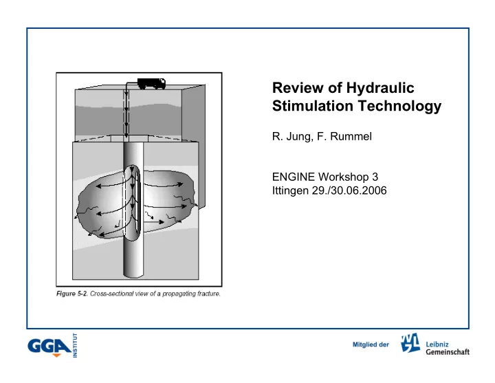
SLIDE 1 Review of Hydraulic Stimulation Technology
ENGINE Workshop 3 Ittingen 29./30.06.2006
SLIDE 2
volume pressure
2 a
Mechanical properties of fractures
SLIDE 3
2 a 0.001-0.01 in contact 3000 3 1000 3 0.3 100 0.003 0.03 10 3·10-6 0.003 1 [m³/bar] [mm/bar] [m] dV/dp dw/dp 2a E = 50 GPa
Mechanical properties of fractures
SLIDE 4
volume pressure
2 a 2 a + 2 ∆a
Mechanical properties of fractures
SLIDE 5
volume pressure
2 a 2 a + 2 ∆a ∆W ≥ 2 ∆a·γ ∆W Griffith (1921)
Fracture propagation
γ : surface energy γ = 10 – 100 J/m²
SLIDE 6
2 a
Fracture propagation r σθ ∝ KI / √r KI = KIC KI = p ·√πa KIC: fracture toughness KIC = 1 MPa·m1/2 Irvin (1958)
SLIDE 7
q = (w3/12)/µ·dp/dx = T/µ·dp/dx w fluid flow in fractures T : fracture transmissibility µ : viscosity
SLIDE 8
fluid flow in fractures
10 10-11 Porous aquifer 105 10-7 10 100 10-10 1 0,1 10-13 0.1 10-4 10-16 0.01 [D·m] [m³] [mm] T T w
w q = (w3/12)/µ·dp/dx = T/µ·dp/dx
SLIDE 9
fluid flow in fractures w dp/dx = q·µ/T
10-4 1 10 0.1 1 1 100 1 0.1 105 1 0.01 [bar/m] [l/(s·m)] [mm] dp/dx q w
SLIDE 10
2 a
High gradients at the fracture tip fluid flow in fractures
SLIDE 11
Perkins, Kern, and Nordgren (PKN) Model Geometry Khristianovich, Zheltov, Geertsma, de Klerk (KGD) Model Geometry f f
h x >>
f f
h x << Hydrodynamic fracture models
SLIDE 12 KGD fracture model (1955, 1969)
G = elastic shear modulus, Pa qi = injection rate, m³/s µ = apparent viscosity, Pa·s E = Young‘s modulus, Pa ν = Poisson’s ratio xf = fracture half length, m hf = Fracture height, m ) 1 ( 2 ν + ⋅ = E G
⋅ ⋅ − ⋅ ⋅ ⋅ = 4 ) 1 ( 27 , 2
4 / 1 2
π ν µ
f f i
h G x q w
f f
h x << Hydrodynamic fracture models
SLIDE 13 PKN fracture model
G = elastic shear modulus, qi = injection rate µ = apparent viscosity E = Young‘s modulus (107 - 2x10⁵ psi) ν = Poisson’s ratio (0,15 - 0,4) xf = fracture half length ) 1 ( 2 ν + ⋅ = E G
⋅ ⋅ − ⋅ ⋅ ⋅ = γ π ν µ 4 ) 1 ( 31 , 2
4 / 1
G x q w
f i
qi = injection rate, bpm µ = apparent viscosity, cp G = elastic shear modulus, psi xf = fracture half length, ft γ = geometry factor app. 0,75 f f
h x >> Hydrodynamic fracture models
SLIDE 14
12 0.75 1000 4 0.25 100 1.2 0.075 10 0.4 0.025 1 wc, [mm] wc, [mm] [m] KDG Griffith 2a
q = 1 l/(s·m) water Hydrodynamic fracture models
Comparision with static fracture models
SLIDE 15 τ − ⋅ ⋅ = t A C q
L L
2
CL= fluid loss coefficient A = element of fracture area t = time measured from pump start τ = time measured from creation of A
Fluid losses
SLIDE 16 − ⋅ + ⋅ ) 1 ( 3 8 2 1 η π η
i p f L L f i i L f i
t r A C K w A t q V V V ⋅ ⋅ ⋅ ⋅ ⋅ + ⋅ = ⋅ + = ) 2 (
qi = injection rate ti = injection time Af = fracture area = average fracture width CL = leakoff coefficient rp = ratio of net to fracture height KL = η = fluid efficiency = Vpad = pad volume not carrying proppants
Volume injected = created fracture volume + fluid leak off
(Nolte)
i f
V V
w
Fluid losses
SLIDE 17
k,s xf T Q = 0.1 l/(s·m) TD = T/k·xf TD = 0.1 post frac tests
SLIDE 18 Test 08h 5000000 10000000 15000000 20000000 25000000 30000000 1 10 100 1000 10000 100000 s Pa
TD = 0.1 post frac tests
SLIDE 19
k,s xf T TD = T/k·xf TD = 1 Q = 0.1 l/(s·m) post frac tests
SLIDE 20 TD = 1 post frac tests
Test 08c 2000000 4000000 6000000 8000000 10000000 12000000 14000000 16000000
0,00 2,00 4,00 6,00 8,00 10,00 12,00 14,00 16,00 18,00
s^(1/4) Pa
SLIDE 21
k,s xf T TD = T/k·xf TD = 10 Q = 0.1 l/(s·m) post frac tests
SLIDE 22 post frac tests
Test 08 g 2000000 4000000 6000000 8000000 10000000 12000000 0,00 2,00 4,00 6,00 8,00 10,00 12,00 14,00 16,00 18,00 s^(1/4) Pa
TD = 10