Results and Applications to Inform Landscape-scale Management How - - PowerPoint PPT Presentation

SLIDE 1

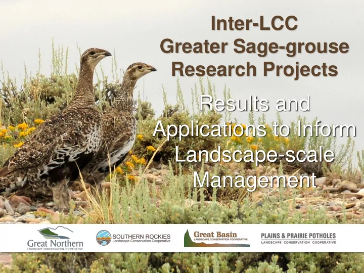
Inter-LCC Greater Sage-grouse Research Projects

Results and Applications to Inform Landscape-scale Management

SLIDE 2

How Did We Get Here?

SLIDE 3

Region 6 Inter-LCC Sage-Grouse Collaboration Proposal

Spoke to a paradigm shift in sage-grouse management

Envisioned paradigm:

– Collaboration among management entities at range-wide and LCC scales – Coordination of planning and implementation to reduce redundancy, target efforts to high priorities and increase efficiency – Management informed by science-based decision support tools – Sage-grouse data shared and available to all through a common data portal – WAFWA as appropriate entity to lead collaborative efforts

SLIDE 4

Collaboration Started with Oversight Committee

• Developed and distributed RFP & scoring criteria
• OC makeup, 23 individuals with science/sage-

grouse expertise or responsibility

– 6 state Division of Wildlife sage-grouse biologists/researchers – 5 LCC Science Coordinators – 7 Federal (FWS, BLM, USFS, USGS) – 3 University Professors – 2 WAFWA (Stiver and Remington)

SLIDE 5

RFP – called for:

• Meaningful impact to sage-grouse conservation

in the short term, completed by 30 Sept. 2015

• Large-scale; at least at scale of single LCC, ideally

multi-LCC

• Research to fill data gaps, mapping, decision

support tools, adaptive management constructs, evaluate effectiveness of current management,

• etc. eligible
• Data must be made available to LC MAP portal,

appropriate protections allowed

SLIDE 6

• 42 proposals received requesting $5.13

million, leveraging over $6 million

• Reviewed and ranked by 13 OC members
• Funding awarded to 4 projects

SLIDE 7

Revisions:

Principal Investigators Title Mike Gregg, FWS Using cheatgrass suppressive soil bacteria to break the fire cycle and proactively maintain greater sage-grouse habitats Collin Homer, USGS Matt Bobo, BLM Annual Grass Cover Mapping for Greater Sage-Grouse Conservation Lyman McDonald Ryan Nielson West, Inc. Analysis of Greater Sage-Grouse Lek Data: Trends in Peak Male Counts, 1965-2015

SLIDE 8

Sage Grouse Hate Trees: A Range-Wide Solution for Increasing Bird Benefits Through Accelerated Conifer Removal

Michael J. Falkowski Colorado State University Department of Ecosystem Science and Sustainability

Collaborators: Aaron Poznanovic (UMN), Dave Naugle (UMT/SGI), Jeremy Maestas (NRCS), Christian Hagen (OSU/LPCI), Jeffery Evans (TNC), Brady Allred (UMT)

SLIDE 9

2 4 6 8 0.0 0.2 0.4 0.6 0.8 1.0 % CONIFER COVER Probability of lek activity

Top down threat with population-level impacts at low levels of tree cover

Baruch-Mordo et al. 2013. Biological Conservation

SLIDE 10

Severson et al., In Review

Sage-Grouse Nesting Impacts

Relative Probability Juniper Cover (%)

SLIDE 11

It’s not just about grouse….

+55% +85%

Sagebrush Obligates of High Conservatio n Concern Holmes et al., In Review Open Woodland Songbird

SLIDE 12

• Tree removal increased available

nesting habitat by 28%

• Probability of use of newly restored

sites increased by 22% annually

• Hens were 43% more likely to nest

within 1000 m of treatments

• 29% of marked birds shifted

nesting into treated habitats

Severson et al., In Review

Does conifer removal work?

SLIDE 13

Source: Dave Naugle - Photos by: Andy Gallagher

Where Are the Trees?

How do we prioritize? Where do we start?

SLIDE 14

A rangewide tool for scaling up implementation

Proposed acres (millions) of conifer mapping by state within PAC and non-PAC areas.

>102 million acres (~413,000 km2) to be mapped

How do we prioritize? Where do we start?

SLIDE 15

Object Based Juniper Detection Can We Determine the Size and Location of Every Tree?

SLIDE 16

We use an object-based image analysis approach (spatial wavelet analysis) to map the location and crown diameter of individual juniper trees in NAIP images, then calculate canopy cover per acre using a moving window. Can also calculate tree density.

Object Oriented Approach: Spatial Wavelet Analysis Applied to NAIP NDVI Image

SLIDE 17

We use an object-based image analysis approach (spatial wavelet analysis) to map the location and crown diameter of individual juniper trees in NAIP images, then calculate canopy cover per acre using a moving window.

Object Oriented Approach: Spatial Wavelet Analysis Applied to NAIP NDVI Image

SLIDE 18

Utah Montana California Idaho Nevada Oregon Colorado Wyoming

240 480 120 Kilometers

Canopy Cover

0 - 01% 01 - 20% 20-50%

>102 million acres (~413,000 km2) mapped

>20%

In Progress

SLIDE 19

Texas Colorado New Mexico Kansas Oklahoma

170 340 85 Kilometers

Canopy Cover

01 - 15% >15% 0 - 01%

>24 million acres (~107,000 km2) mapped

SLIDE 20

In 5 years - 405,241 Acres Treated Highly targeted to prioritized populations - 81% in PACs

Population % Threat reduced SGI 1.0 Central Oregon 85% Northern Great Basin 67% Western Great Basin 52% Baker, Oregon 41% TOTAL 68%

SGI Conifer Removal inside PACs

Or Oreg egon n Exampl mple

Strategic approach to threat alleviation

SLIDE 21

targeting implementation and outcomes putting data into the right hands

SLIDE 22

Prioritizing conifer removal for Sage Grouse conservation

Where to target removal?

• Costly
• Limited Resources
• Most beneficial areas?
• Oregon Case Study

SLIDE 23

SLIDE 24

SLIDE 25

SLIDE 26

Thanks !! Funding Sources and Cooperators:

Conifer mapping in the sage grouse range was supported by a grant administered by the Western Association of Fish and Wildlife Agencies (WAFWA) with funding partners including the: U.S. Fish and Wildlife Service Bureau of Land Management National Fish and Wildlife Foundation Utah Department of Natural Resources - Watershed Restoration Initiative Special Thanks to TNC

SLIDE 27

Designing a regional network of fuel breaks to protect Greater Sage-Grouse habitat: An experimental approach using Circuitscape

Nathan Welch (ID), Louis Provencher (NV), Bob Unnasch (ID), Tanya Anderson (NV) & Brad McRae (North America)

27

SLIDE 28

29

“Create and maintain effective fuel breaks in strategic locations that will modify fire behavior and increase fire suppression effectiveness….” “Federal firefighters shall ensure close coordination with State firefighters, local fire departments and local expertise (i.e., livestock grazing permittees and road maintenance personnel) to create the best possible network of strategic fuel breaks and road access to minimize and reduce the size

• f a wildfire following

ignition…”

SLIDE 29

• Policy documents identify the need for landscape-scale approaches to

design and implement fuel treatments to stop or slow fire spread.

• We developed a GIS protocol for identifying strategic

locations for fuel breaks at large spatial extents and simulating potential fuel breaks.

• We proposed next steps in the refinement of our

protocol and devised general recommendations for a regional network of fuel breaks to prevent loss of critical Sage-Grouse habitat.

31

Response

Ken Miracle

SLIDE 30

32

SLIDE 31

Methods

• We simulated wildfire transmission / fuel break potential using

Circuitscape, which is based on electrical circuit theory.

• The inputs for the model are sources where electrical current

enters the system (=ignitions), grounds where current departs the system (=edge of the landscape), and a resistance surface (=flammability raster) across which the current will flow between sources and grounds.

• We identified “pinch points” that provide connections between

areas with high flammability, but where adjacent areas with low flammability could constrict wildfire.

• We installed sample fuel breaks in “pinch point” areas and

simulated fuel break behavior by modifying the sources raster to include negative current sources that remove fire from the system.

34

SLIDE 32

35

SLIDE 33

36

SLIDE 34

37

Creating the Resistance Raster

SLIDE 35

38

SLIDE 36

39

SLIDE 37

40

SLIDE 38

41

SLIDE 39

42

SLIDE 40

44

Run Circuitscape

SLIDE 41

45

SLIDE 42

Interpreting Circuitscape Results

46

SLIDE 43

Cheatgrass

(very high flammability)

In this landscape, locations A and B have the same wildfire likelihood.

Lek

A B

47

SLIDE 44

In this landscape, Circuitscape tells us locations A and B have the same current density (= wildfire transmission or fuel break potential).

Lek

A B

48

SLIDE 45

Cheatgrass

(very high flammability)

Alfalfa

(very low flammability)

Lek

A B

In this new landscape, locations A and B still have roughly the same wildfire likelihood.

49

SLIDE 46

A B

However, now Circuitscape tells us locations A and B have very different current densities (= wildfire transmission or fuel break potential). The area surrounding B is a “pinch point” and might be a more efficient place for a fuel break.

Lek

50

SLIDE 47

51

SLIDE 48

52

SLIDE 49

53

SLIDE 50

54

SLIDE 51

55

SLIDE 52

56

SLIDE 53

57

SLIDE 54

58

• Using Circuitscape, we have developed a process to identify

strategic locations for fuel breaks at regional scales and to simulate potential fuel breaks with different levels of effectiveness (i.e., permeability). It provides a starting place for land managers to consider in planning efforts. It does not indicate whether a fuel break is possible, practical, or desirable from a local perspective.

• Our report is being shared with public and private land

managers as another resource to inform decisions about land and fire management. We intend to pursue a collaboration with fire managers in at least one of the focal geographies we identified.

• We are pursuing opportunities to test and improve our

modeling approach and to conduct a rigorous comparison with more sophisticated fire models.

Next Steps

SLIDE 55

59

We are grateful for funding from the Western Association of Fish and Wildlife Agencies and, ultimately, to the U.S. Fish and Wildlife Service. Elaine York (The Nature Conservancy in Utah) and Jay Kerby (The Nature Conservancy in Oregon) helped with local agency workshop coordination and outreach.

Acknowledgments

SLIDE 56

60

I’m a Fire-on

SLIDE 57

U.S. Department of the Interior U.S. Geological Survey

Collin Homer, April 4th, 2016

Characterization of Shrub/Grass Components Across the West with Remote Sensing, New Opportunities for Habitat and Trend Analysis

SLIDE 58

Outline and Acknowledgments

• What are remote sensing components and how are

they created?

• What are the current results?
• How can they be used?
• What products are coming?
• Future possibilities?
• How to get them

Acknowledgements:

• Many individuals doing this work at USGS-EROS, USGS-FRESC and USGS-

FORT and BLM, USGS and WAFWA/USFWS for providing funding

SLIDE 59

What are fractional vegetation components?

1 Meter Frame Component proportions are field measured and then extrapolated to satellite imagery pixels in the same way

Vegetation Components

• Sagebrush/shrub - 30%
• Herbaceous - 15%
• Litter - 10%
• Bare ground - 45%

SLIDE 60

Fractional components are scaled up from field measurements with 2 scales of satellite imagery using regression tree models

Landsat Bare Ground (30meter pixel) High Resolution Satellite Bare Ground (2.4 meter pixel) Field Measured Bare Ground State of Wyoming

SLIDE 61

Products require extensive fieldwork at strategic Worldview 2/3 collects to be successful (about 144 sq. km. each)

SLIDE 62

All Sage Cover (%)

Value

High : 102 Low : 0

Annual Herbaceous Cover (%)

Value

High : 102 Low : 0

Bare Ground (%)

Value

High : 102 Low : 0

All Sage Height (cm)

Value

High : 178 Low : 0

All Shrub Height (cm)

Value

High : 428 Low : 0

All Sage Cover (%)

Value

High : 102 Low : 0

Annual Herbaceous Cover (%)

Value

High : 102 Low : 0

Bare Ground (%)

Value

High : 102 Low : 0

All Sage Height (cm)

Value

High : 178 Low : 0

All Shrub Height (cm)

Value

High : 428 Low : 0

All Sage Cover (%)

Value

High : 102 Low : 0

Annual Herbaceous Cover (%)

Value

High : 102 Low : 0

Bare Ground (%)

Value

High : 102 Low : 0

All Sage Height (cm)

Value

High : 178 Low : 0

All Shrub Height (cm)

Value

High : 428 Low : 0

All Sage Cover (%)

Value

High : 102 Low : 0

Annual Herbaceous Cover (%)

Value

High : 102 Low : 0

Bare Ground (%)

Value

High : 102 Low : 0

All Sage Height (cm)

Value

High : 178 Low : 0

All Shrub Height (cm)

Value

High : 428 Low : 0

All Sage Cover (%)

Value

High : 102 Low : 0

Annual Herbaceous Cover (%)

Value

High : 102 Low : 0

Bare Ground (%)

Value

High : 102 Low : 0

All Sage Height (cm)

Value

High : 178 Low : 0

All Shrub Height (cm)

Value

High : 428 Low : 0

Herbaceous Cover (%)

Value

High : 102 Low : 0

All Shrub Height (cm)

Value

High : 428 Low : 0

Litter Cover (%)

Value

High : 102 Low : 0

All Shrub Height (cm)

Value

High : 428 Low : 0

Big Sage Cover (%)

Value

High : 102 Low : 0

All Shrub Cover (%)

Value

High : 102 Low : 0 High : 100 Low : 0 High : 100 Low : 0 High : 100 Low : 0 High : 100 Low : 0 High : 100 Low : 0 High : 100 Low : 0 High : 100 Low : 0

9 Shrub component products are being produced

Values in 1% increments

SLIDE 63

Mask Mask Mask

Shrub Prediction Bare Ground Prediction Shrub Absolute Error Bare Ground Absolute Error

Mask

Validation includes independent validation, cross validation and a spatial absolute error model prediction with all products

SLIDE 64

Great Basin Percent Sagebrush Component

RMSE accuracy is about 6%

SLIDE 65

Great Basin Annual Herbaceous Component

RMSE accuracy is about 7%

SLIDE 66

The component approach provides maximum flexibility to compile components for endless applications – such as:

• Sage grouse habitat (Wyoming state-wide seasonal

models (Fedy et al., 2014), and new habitat modeling across Great Basin)

• Grazing assessment (Wyoming grazing assessment

showing differences in allotments that failed LHS)

• Invasives (used for monitoring cheatgrass growth
• ver Twin Falls Idaho and Winnemucca Nevada)
• Climate change (used to quantify vegetation change

in response to climate in Wyoming and Nevada)

• As well as other applications in fire fuel analysis,

restoration monitoring, other climate impacts

SLIDE 67

1993 1997 2004 2009 2011

Nevada example

• f quantifying

cheatgrass increase over time, 1993-2011

White – masked out areas

SW of Hot Springs Range

Cheatgrass quantity The component approach allows better quantification and monitoring of change

SLIDE 68

Average yearly value in climate changed pixels for Northwest Nevada/Southeast Oregon, 1985-2014

The Landsat archive can be used to see components change over time, such as this climate example… Steppe area

SLIDE 69

That historical relationship can then be modeled for each pixel…..

1984-2011 Annual Precipitation Trend Linear Regression 1984-2011 Annual Sagebrush Component Trend

SLIDE 70

Each pixel model can then forecasted into the future

2050 sagebrush projected cover from projected precipitation slope for a selected pixel

Regression between sagebrush cover and annual precipitation for a selected pixel

History Future

SLIDE 71

This approach was used to predict the impact of climate change

• n Sage grouse

nesting habitat between 2006 and 2050 – results indicate an 11% overall loss…..

Homer, C, Xian, G., Aldridge, C., Meyer, D., Loveland, T. and M. O’Donnell. 2015. Forecasting sagebrush ecosystem components and greater sage-grouse habitat for 2050: Learning from past climate patterns and Landsat imagery to predict the future. Ecological Indicators, Vol. 55, 131–145.

SLIDE 72

Research Goals – tell this story about every pixel in the West…..

• Characterize it’s components
• Score the “intactness” of the pixel against expected

site potential

• Determine how much the pixel changed since 1983,

and what caused the change?

• How much of that change is climate?
• Knowing the past history, what is the likely future

trend for the pixel from climate and other change agents?

• Communicate results with interactive data “maps”

SLIDE 73

Total area mapped after 2016 field season

Field sampled high resolution satellite areas in red (189) Independent validation plots in black (1,475)

SLIDE 74

NLCD is a Landsat derived 30m suite of land cover products covering the United States created by 10 Federal partners (Multi-Resolution Land Characteristics Consortium)

Great Basin components available on the MRLC website www.mrlc.gov on April 15th

Products

SLIDE 75

Environmental & Statistical Consultants

Trends in Lek Attendance by Male Greater Sage-Grouse

Ryan Nielson Lyman McDonald Jason Mitchell Shay Howlin Chad LeBeau

4/4/2016

SLIDE 76

WEST, Inc.

| 80 |

An Independent Look

• Trends in peak (max) lek attendance by males

1965 – 2015.

• There have been other analyses.

SLIDE 77

WEST, Inc.

| 81 |

An Independent Look

• WEST was asked to
• Recommend an analysis approach.
• Provide an example of the analysis using

historic data (1965-2015).

SLIDE 78

WEST, Inc.

| 82 |

An Independent Look

• Our recommendations:
• Keep analysis assumptions to a minimum.
• Avoid transformation of the data.
• Follow individual leks through time.

SLIDE 79

WEST, Inc.

| 83 |

Analysis Approach

• Lek = 2 or more males in 2 or more years
• Data from larger leks + spatially related

satellite leks or activity centers were combined.

– Clustering analysis combined counts within 1.2-km into lek complexes

SLIDE 80

WEST, Inc.

| 84 |

Analysis Approach

• Follow standard of not including portions of

lek counts with large strings of zeros.

14, 5, 9, 11, 4, 0, 0, 0, 0, 0, 0, 3, 5,…

• An artifact of the way individual States and

biologists treat individual leks and record data.

SLIDE 81

WEST, Inc.

| 85 |

Analysis Approach

• Applied a well-developed model that has been peer-

reviewed and published

• Thogmartin et al. (2006, Condor)
• Nielson et al. (2008, The Auk)
• Sauer and Link (2011, The Auk)
• Millsap et al. (2013, JWM)
• Nielson et al. (2014, JWM)

SLIDE 82

WEST, Inc.

| 86 |

Analysis Approach

• Bayesian Hierarchical Model
• Follows individual leks through time.
• Trends for individual management zones.
• Overall trend.
• Analyze entire management zone, core area,

and periphery.

SLIDE 83

WEST, Inc.

| 87 |

Management Zones

SLIDE 84

WEST, Inc.

| 88 |

75% Core Area

SLIDE 85

WEST, Inc.

| 89 |

What is a Trend?

SLIDE 86

WEST, Inc.

| 90 |

Results

SLIDE 87

WEST, Inc.

| 91 |

Results

SLIDE 88

WEST, Inc.

| 92 |

Results

SLIDE 89

WEST, Inc.

| 93 |

Results

SLIDE 90

WEST, Inc.

| 94 |

Results

SLIDE 91

WEST, Inc.

| 95 |

Results

SLIDE 92

WEST, Inc.

| 96 |

Results

SLIDE 93

WEST, Inc.

| 97 |

Results

• Average of a 1.3% decline per year (core area)

across the 7 management zones.

• Ignore zones 1 and 6 … <0.9% decline per year

SLIDE 94

WEST, Inc.

| 98 |

Results

SLIDE 95

WEST, Inc.

| 99 |

Results

SLIDE 96

WEST, Inc.

| 100 |

Analysis Limitations

• Varying survey effort within management zones /

states and between years. – More consistency 2007 – present.

• Somewhat opportunistic sampling, especially in the

early years.

• Early years focused more on larger leks?
• Handling of zeros

14, 5, 9, 11, 4, 0, 0, 0, 0, 0, 0, 0, 0,… OR 14, 5, 9, 11, 4, 0, 0, 0, 0, 0, 0, 2, 6,…

SLIDE 97

WEST, Inc.

| 101 |

Analysis Limitations

• Probability of detection.
• Not part of a probability-based sample of leks.
• Rate of change in males on leks may not be the best

metric for rate of change on population size. – Maybe OK for estimating direction of trends. – LPC surveys have seen increases in abundance with decreases in lek size.

SLIDE 98

WEST, Inc.

| 102 |

Recommendations

• Use the Bayesian Hierarchical Model described

above for retrospective looks.

• Report can be found on the WEST and WAFWA

websites.

• Develop a user-friendly analysis tool with a simple

dashboard.

– Requires common storage and filtering of data.

SLIDE 99

WEST, Inc.

| 103 |

Future Analyses

• Range-wide population abundance survey during

winter/breeding.

• Monitoring efforts and data storage consistent over

time and space.

• Develop regional RSFs to identify key landscape

characteristics.

• Keep assumptions to a minimum.

SLIDE 100

west-inc.com

307.634.1756 415 West 17th Street, Suite 200, Cheyenne, WY 82001 Corporate Headquarters

SLIDE 101

IMPROVING POPULATION SIZE AND TREND ESTIMATION IN GREATER SAGE-GROUSE

Paul M. Lukacs Rebecca McCaffery

• J. Josh Nowak

SLIDE 102

Objectives:

• Improve sampling design
• Develop an integrated population model
• Design user-friendly software for to

implement analyses

SLIDE 103

Our approach

• Lek counts

– Can we re-think the use of lek data to improve abundance estimation?

• Population models

– Combine multiple sources of information

• Software

– Capitalize on the power of shared computing and ease of web platforms

SLIDE 104

N-Mixture Models

• Male grouse per lek (biological process)

– 𝑂𝑗𝑙 ~ Poisson(λ𝑗𝑙 )

• Variation in lek size

– log λ𝑗𝑙 = α𝑗 + 𝑠

𝑗 𝑙 − 1 + ε𝑗

SLIDE 105

N-Mixture Models

• Lek counts (observed data)

– 𝑧𝑗𝑘𝑙 𝑂𝑗𝑙 ~ Bin(𝑂𝑗𝑙, 𝑞𝑗𝑘𝑙)

• Variation in detection probability

– logit 𝑞𝑗𝑘𝑙 = α𝑗𝑘𝑙 + β𝑥 × 𝑦𝑗𝑘𝑙𝑥 + δ𝑗𝑘𝑙

SLIDE 106

N-Mixture Models

• Key features

– Allows variation in lek size as a function of environmental features – Allows variation in detection as a function of

• bserver or lek-specific characteristics

SLIDE 107

N-Mixture Models

• Do N-mixture models adequately estimate

abundance from lek count data?

• If they work, how frequently do we have to

sample leks?

SLIDE 108

Results-simulation

SLIDE 109

Percent missing data SD of population growth rate

Precision: Variable p:

SLIDE 110

Case Study - Montana

• Lek counts from 2002-2014
• Multiple counts per lek (at some leks)
• Not all leks surveyed in all years

SLIDE 111

Variation in detection probability over time

Detection probability Year Where population growth rate is explicitly included in the model

SLIDE 112

N-mixture model estimate High male count Year Year Mean lek abundance Case study: State of Montana 2002-2014:

• a. Mean annual lek size
• b. Population trend explicitly

included in model

SLIDE 113

N-mixture model

• Summary

– Useful for improving estimation from lek counts – Includes the detection probability – Guides sampling design

SLIDE 114

Integrated Population model

• Combine multiple sources of information

– Lek counts – Survival – Recruitment – Sex ratio

SLIDE 115

IPM insights

• Lek counts may overstate variation in

abundance

• Absence of sex ratio estimates is limiting

inference

SLIDE 116

Population Growth Rate (λ)

Raw Lek Counts N-mixture Estimates

SLIDE 117

Software

SLIDE 118

PopR

SLIDE 119

PopR

SLIDE 120

PopR

SLIDE 121

IPM

• Summary

– Model provides framework to consider data collection – Guides synthesis of multiple sources of data – PopR provides a workflow to simplify the modelling process

SLIDE 122

Summary

• Sampling Design

– Better to survey more leks less frequently – Visit leks you do survey more than once per year and record the data in a database

• Population Models

– Reduce sampling variation in population trajectory – Demonstrate need for sex ratio estimates

• PopR

– Easy to use, web-based software

SLIDE 123

Questions?