reservoir computing in the time domain
play

Reservoir Computing in the Time Domain Laurent Larger, Antonio - PowerPoint PPT Presentation

Reservoir Computing in the Time Domain Laurent Larger, Antonio Bayln-Fuentes, Romain Martinenghi, Vladimir S. Udaltsov, Yanne K. Chembo and Maxime Jacquot, High-Speed Photonic Reservoir Computing Using a Time-Delay-Based Architecture: Million


  1. Reservoir Computing in the Time Domain 
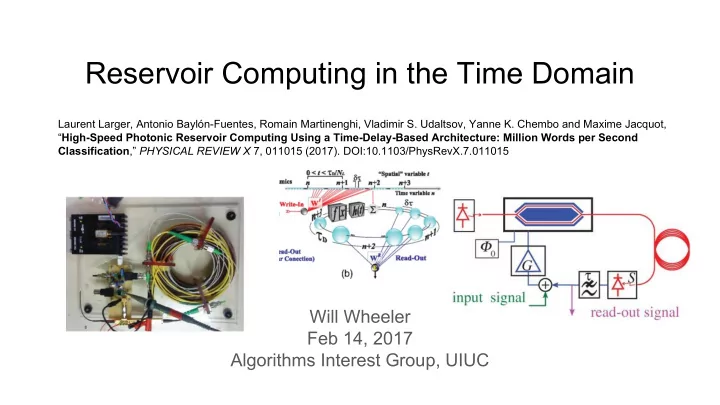
Laurent Larger, Antonio Baylón-Fuentes, Romain Martinenghi, Vladimir S. Udaltsov, Yanne K. Chembo and Maxime Jacquot, “ High-Speed Photonic Reservoir Computing Using a Time-Delay-Based Architecture: Million Words per Second Classification ,” PHYSICAL REVIEW X 7, 011015 (2017). DOI:10.1103/PhysRevX.7.011015 Will Wheeler Feb 14, 2017 Algorithms Interest Group, UIUC

  2. We want greater computing power Turing-von Neumann architecture: can’t we Brains are good: let’s make computers like do better? brains. Neural network simulation! Still not how brains work, but this has ...Wait, this isn’t how brains work dynamics (cycles)

  3. Reservoir computing Nonlinear function Nonlinear dynamical system With each sample: With each sample: ⋄ Train input weights ⋄ Fixed input weights Train hidden weights Fixed hidden weights ⋄ ⋄ ⋄ Train output weights ⋄ Train output weights Romain Modeste Nguimdo, Guy Verschaffelt, Jan Danckaert, and Guy Van der Sande, "Reducing the http://cs231n.github.io/neural-networks-1/ phase sensitivity of laser-based optical reservoir computing systems," Opt. Express 24 , 1238-1252 (2016)

  4. Time domain of a single node Principles of RC, with an input mask WI spreading the input information onto the RC nodes, and with a read-out WR extracting the computed output from the node states. Left diagram: A spatially extended dynamical network of nodes. Right diagram: A nonlinear delayed feedback dynamics emulating virtual nodes which are addressed via time multiplexing. Here, f(x) stands for the nonlinear feedback transformation, and h(t) denotes the loop linear impulse response. Romain Modeste Nguimdo, Guy Verschaffelt, Jan Danckaert, and Guy Van der Sande, "Reducing the phase sensitivity of laser-based optical reservoir computing systems," Opt. Express 24 , 1238-1252 (2016)

  5. Time multiplexing feedback delay time τ D input vectors N L τ D /N L τ D /N L τ D /N L K elements per τ D /(N L K) τ D /(N L K) τ D /(N L K) τ D /(N L K) τ D /(N L K) τ D /(N L K) τ D /(N L K) τ D /(N L K) τ D /(N L K) τ D /(N L K) τ D /(N L K) τ D /(N L K) input vector Discrete time variables n (input vector) σ (input element) Time-scale of dynamics: about 5 input units

  6. System implementation with laser demodulator has “time imbalance δT” form of interference function EO phase setup involving two integrated optic phase modulators followed by an imbalanced Mach-Zehnder DPSK demodulator providing a temporally nonlocal, nonlinear, phase-to-intensity conversion. The information to be processed by this delay photonic reservoir is provided by a high-speed arbitrary waveform generator (AWG). The response signal from the delay dynamics is recorded by an ultrafast real-time digital oscilloscope at the bottom of the setup, after the circulator, followed by an amplified photodiode and a filter.

  7. Input data Data from the TI46 speech corpus: 500 pronounced digits between 0 and 9. The digits are pronounced by five different female speakers uttering the 10 digits 10 times, with the acoustic waveform being digitally recorded at a sampling rate of 12.5 kHz. Cochleagram: 1D sound waveform → 2D frequency-time matrix Q frequency channels (rows), N times (cols) [K × Q] [Q × N] [K × N] Illustration of the input information injection into the dynamics. The (sparse and random) K×Q write-in matrix WI performs a spreading of the input cochleagram information represented as a Q×N cochleagram matrix Mu. The resulting K×N matrix Min defines a scalar temporal waveform uIσ(n) obtained after horizontally queuing the N columns, each of them being formed by the K amplitudes addressing the virtual nodes in one layer.

  8. Training readout Asynchronous readout ⋄ Sampling the reservoir is measuring each node. Once the inputs are in, the time scale doesn’t matter! ⋄ We can adjust the time for readout (better performance) ⋄ M=10 classes K nodes N input vectors [M × K] [K × N] [M × N] Illustration of the expected optimized read-out processing through a (M×K) matrix WR, left multiplying the transient response (K×N) matrix Mx, thus resulting in an easy-to-interpret target (M×N) matrix My. The latter matrix is aimed at designating the right answer for the digit to be identified (the second line in this example, indicating digit “1”).

  9. Output data Example of an imperfect “reservoir-computed” target answer while testing the optimal read-out WRopt on an untrained digit of response Mx. However, the digit “2” clearly appears as the most obvious answer for this untrained tested digit. [M × K] [K × N] [M × N]

  10. Interpreting output Illustration of the decision procedure for the computed answer. The temporal amplitudes of the actual target are summed over time for each line (or modality), i.e., for each of the 10 possible digits. The right modality is then declared as the one with the highest sum.

  11. Results WER = word error rate Numerical and experimental results for the parameter optimization with the TI46 database. (a) The cos 2 static nonlinear transformation function and its scanned portion in red, under the best operating points close to a minimum or a maximum. (b) WER vs β parameter, under synchronous write-in and read-out, i.e., δτ/δτ R . The red line is the numerics; the blue line is experimental (best: 1.3%). (c) WER as a function of the relative readout vs write-in asynchrony quantified as ε=δτ R /δτ−1 . (d) WER vs the β parameter, under asynchronous write-in and read-out. The red line is the numerics; the blue line is experimental (best: 0.04%).

  12. My Python simulation is really slow

  13. My Python simulation ...uses The MNIST database of handwritten digits, which are 28×28 pixels grey scale. Training set: 500 Testing set: 20 Great statistics :) http://yann.lecun.com/exdb/mnis t/

  14. My Python simulation - result

  15. My Python simulation - result First column: yellow square is the right answer Second column: result (the sum of each row) Third column: separator between samples Yellow are correct, green are wrong

  16. My Python simulation - does it do anything? This shouldn’t really work: What happens if we eliminate the reservoir? No optimized parameters (β, ρ, Φ 0 , dτ R ) ⋄ Transform the inputs and directly apply optimized Run in python ⋄ output matrix ⋄ Trained on 150 samples This is less good than with the dynamics. It’s useful!

  17. My Python simulation - improvements I’ll post the code on github. You can look at it, run it overnight, or make improvements ⋄ It’s really easy to parallelize over samples It uses a slow integrator ⋄ ⋄ It wasn’t optimized for anything

  18. Thanks! ● Layered neural networks are functions; recurrent neural networks are dynamic systems ● A recurrent neural network can be represented in the time domain of a single nonlinear system ● This can be implemented with lasers for really fast processing ● The lasers can be simulated in python really slowly ● But the paper’s authors have real simulations to optimize parameters and check performance

Download Presentation
Download Policy: The content available on the website is offered to you 'AS IS' for your personal information and use only. It cannot be commercialized, licensed, or distributed on other websites without prior consent from the author. To download a presentation, simply click this link. If you encounter any difficulties during the download process, it's possible that the publisher has removed the file from their server.

Recommend


More recommend