Reinforcement Learning n-armed bandit Kevin Spiteri April 21, 2015 - PowerPoint PPT Presentation

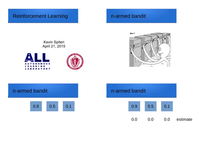
Reinforcement Learning n-armed bandit Kevin Spiteri April 21, 2015 n-armed bandit n-armed bandit 0.9 0.5 0.1 0.9 0.5 0.1 0.0 0.0 0.0 0.0 estimate

n-armed bandit n-armed bandit 0.9 0.5 0.1 0.9 0.5 0.1 0 0.0 0.0 0.0 0.0 estimate 1.0 0.0 0.0 1.0 0.0 0.0 estimate 0 0 0 0.0 0 attempts 1 0 0 1 0.0 0 attempts 0 0 0 0.0 0 payoff 1 0 0 1 0.0 0 payoff n-armed bandit Exploration 0.9 0.5 0.1 0.9 0.5 0.1 0.5 0.0 1.0 0.5 0.0 0.0 estimate 0.67 0.0 1.0 0.5 0.0 0.0 estimate 2 0 1 2 0.0 0 attempts 3 0 1 2 0.0 0 attempts 1 0 1 1 0.0 0 payoff 2 0 1 1 0.0 0 payoff

Going on … Changing environment 0.9 0.5 0.1 0.7 0.8 0.1 0.86 0.9 0.5 0.1 0.0 estimate 0.86 0.9 0.5 0.0 0.1 estimate 300 280 10 0.0 10 attempts 300 280 10 0.0 10 attempts 258 252 5 0.0 1 payoff 258 252 5 0.0 1 payoff Changing environment Changing environment 0.7 0.8 0.1 0.7 0.8 0.1 0.77 0.8 0.65 0.0 0.1 estimate 0.72 0.74 0.74 0.1 0.0 estimate 600 560 20 0.0 20 attempts 1500 1400 50 0.0 50 attempts 463 448 13 0.0 2 payoff 1078 1036 37 0.0 5 payoff

n-armed bandit n-armed bandit ● Evaluation vs instruction. ● Optimal payoff (0.82): ● Discounting. 0.9 x 300 + 0.8 x 1200 = 1230 ● Initial estimates. ● Actual payoff (0.72): 0.9 x 280 + 0.5 x 10 + 0.1 x 10 + ● There is no best way or standard way. 0.7 x 1120 + 0.8 x 40 + 0.1 x 40 = 1078 Markov Decision Process Markov Decision Process (MDP) (MDP) ● States

Markov Decision Process Markov Decision Process (MDP) (MDP) ● States ● States ● Actions c b a Markov Decision Process Markov Decision Process (MDP) (MDP) ● States ● States ● Actions ● Actions c c ● Model ● Model a 0.75 a 0.75 b b a 0.25 a 0.25

Markov Decision Process Markov Decision Process (MDP) (MDP) ● States ● States ● Actions ● Actions c c 0 0 ● Model ● Model ● Reward ● Reward a 0.75 a 0.75 5 5 -1 -1 ● Policy b b a 0.25 a 0.25 Markov Decision Process Markov Decision Process (MDP) (MDP) ● States: ball ● States: ball table table hand hand t t h t h basket basket floor floor b f b f

Markov Decision Process Markov Decision Process (MDP) (MDP) ● States: ball ● States: ball table table c c hand hand t h t h basket basket floor floor ● Actions: ● Actions: a 0.75 b b a a 0.25 a) attempt a) attempt b f b f b) drop b) drop c) wait c) wait Markov Decision Process Markov Decision Process (MDP) (MDP) ● States: ball ● States: ball table table c c 0 hand hand t h t h basket basket floor floor ● Actions: a 0.75 ● Actions: a 0.75 5 -1 b b a 0.25 a 0.25 a) attempt a) attempt b f b f b) drop b) drop c) wait c) wait

Markov Decision Process Markov Decision Process (MDP) (MDP) ● States: ball ● States: ball table table c c 0 0 hand hand -1 t h t h basket basket floor floor ● Actions: a 0.75 ● Actions: a 0.75 5 5 -1 -1 b b a 0.25 a 0.25 a) attempt a) attempt b f b f b) drop b) drop c) wait c) wait Expected reward per round: 0.25 x 5 + 0.75 x (-1) = 0.5 Markov Decision Process Reinforcement Learning (MDP) Tools ● States: ball table ● Dynamic Programming c 0 hand -1 t h basket ● Monte Carlo Methods floor ● Actions: a 0.75 5 -1 b a 0.25 a) attempt ● Temporal Difference Learning b f b) drop c) wait

Grid World Optimal Policy Reward: Normal move: -1 Over obstacle: -10 Best reward: -15 Value Function Initial Policy -15 -8 -7 0 -14 -9 -6 -1 -13 -10 -5 -2 -12 -11 -4 -3

Policy Iteration Policy Iteration -21 -11 -10 0 -21 -11 -10 0 -22 -12 -11 -1 -22 -12 -11 -1 -23 -13 -12 -2 -23 -13 -12 -2 -24 -14 -13 -3 -24 -14 -13 -3 Policy Iteration Policy Iteration -21 -11 -10 0 -22 -12 -11 -1 -23 -13 -12 -2 -24 -14 -13 -3

Policy Iteration Policy Iteration -21 -11 -10 0 -21 -11 -10 0 -22 -12 -11 -1 -22 -12 -11 -1 -23 -13 -12 -2 -23 -13 -12 -2 -15 -14 -4 -3 -15 -14 -4 -3 Policy Iteration Policy Iteration -21 -11 -10 0 -22 -12 -11 -1 -23 -13 -12 -2 -15 -14 -4 -3

Policy Iteration Value Iteration -15 -8 -7 0 0 0 0 0 -14 -9 -6 -1 0 0 0 0 -13 -10 -5 -2 0 0 0 0 -12 -11 -4 -3 0 0 0 0 Value Iteration Value Iteration -1 -1 -1 0 -2 -2 -2 0 -1 -1 -1 -1 -2 -2 -2 -1 -1 -1 -1 -1 -2 -2 -2 -2 -1 -1 -1 -1 -2 -2 -2 -2

Value Iteration Value Iteration -3 -3 -3 0 -15 -8 -7 0 -3 -3 -3 -1 -14 -9 -6 -1 -3 -3 -3 -2 -13 -10 -5 -2 -3 -3 -3 -3 -12 -11 -4 -3 0.95 Stochastic Model Value Iteration 0.025 0.025 -19.2 -10.4 -9.3 0 0.95 -18.1 -12.1 -8.2 -1.5 0.025 0.025 -17.0 -13.6 -6.7 -2.9 -15.7 -14.7 -5.1 -4.0

0.95 Value Iteration Richard Bellman 0.025 0.025 E.g. 13.6: -19.2 -10.4 -9.3 0 13.6 = 0.950 x 13.1 + -18.1 -12.1 -8.2 -1.5 0.025 x 27.0 + 0.025 x 16.7 -17.0 -13.6 -6.7 -2.9 16.6 = -15.7 -14.7 -5.1 -4.0 0.950 x 16.7 + 0.025 x 13.1 + 0.025 x 15.7 Reinforcement Learning Bellman Equation Tools ● Dynamic Programming ● Monte Carlo Methods ● Temporal Difference Learning

0.95 Monte Carlo Methods Monte Carlo Methods 0.025 0.025 0.95 0.025 0.025 0.95 0.95 Monte Carlo Methods Monte Carlo Methods 0.025 0.025 0.025 0.025 -32 -22 -10 0 -21 -11

0.95 0.95 Monte Carlo Methods Monte Carlo Methods 0.025 0.025 0.025 0.025 -21 -11 -10 0 0.95 0.95 Monte Carlo Methods Q-Value 0.025 0.025 0.025 0.025 -32 -10 0 -15 -10 -31 -21 -11 -8 -20

Bellman Equation Learning Rate ● We do not replace an old Q value with a new one. ● We update at a designed learning rate. ● Learning rate too small: slow to converge. ● Learning rate too large: unstable. -15 -10 ● Will Dabney PhD Thesis: Adaptive Step-Sizes for Reinforcement Learning. -8 -20 Reinforcement Learning Richard Sutton Tools ● Dynamic Programming ● Monte Carlo Methods ● Temporal Difference Learning

Temporal Difference Temporal Difference Learning Learning Temporal Difference: ● Dynamic Programming: ● Learn a guess from other guesses Learn a guess from other guesses (Bootstrapping). (Bootstrapping). ● Learn without knowing model. ● Works with longer episodes than Monte ● Monte Carlo Methods: Carlo methods. Learn without knowing model. Temporal Difference 0.95 Monte Carlo Methods Learning 0.025 0.025 Monte Carlo Methods: ● First run through whole episode. -32 -10 0 ● Update states at end. -31 -21 -11 Temporal Difference Learning: ● Update state at each step using earlier guesses.

0.95 0.95 Monte Carlo Methods Temporal Difference 0.025 0.025 0.025 0.025 -19 -10 -32 -10 0 0 -22 -18 -12 -31 -21 -11 0.95 0.95 Temporal Difference Temporal Difference 0.025 0.025 0.025 0.025 23 = 1 + 22 -19 -10 -19 -10 -23 -10 0 -23 -10 0 28 = 10 + 18 -22 -18 -12 -22 -18 -12 -28 -21 -11 -28 -21 -11 21 = 10 + 11 11 = 1 + 10 10 = 10 + 0

Function Approximation Mountain Car Problem ● Most problems have large state space. ● We can generally design an approximation for the state space. ● Choosing the correct approximation has a large influence on system performance. Mountain Car Problem Function Approximation ● Car cannot make it to top. ● We can partition state space in 200 x 200 grid. ● Can can swing back and forth to gain ● Coarse coding – different ways of momentum. partitioning state space. ● We know x and ẋ. ● We can approximate V = w T f ● x and ẋ give an infinite state space. ● E.g. f = ( x ẋ height ẋ 2 ) T ● Random – may get to top in 1000 steps. ● We can estimate w to solve problem. ● Optimal – may get to top in 102 steps.

Problems with Checkers Reinforcement Learning ● Arthur Samuel (IBM) 1959 Policy sometimes gets worse: ● Safe Reinforcement Learning (Phil Thomas) guarantees an improved policy over the current policy. Very specific to training task: ● Learning Parameterized Skills Bruno Castro da Silva PhD Thesis TD-Gammon Deep Learning: Atari ● Neural networks and temporal difference. ● Inputs: score and pixels. ● Current programs play better than human ● Deep learning used to discover features. experts. ● Some games ● Expert work played at super- in input human level. selection. ● Some games played at mediocre level.