Regression Diagnostics and the Forward Search 1 A. C. Atkinson, - - PDF document

Regression Diagnostics and the Forward Search 1

• A. C. Atkinson, London School of Economics

February 23 2009

The first section introduces the ideas of regression diagnostics for check- ing regression models and shows how deletion diagnostics may fail in the presence of several similar outliers. Section 2 describes the forward search for regression models and illustrates several of its properties.

1 Regression Diagnostics

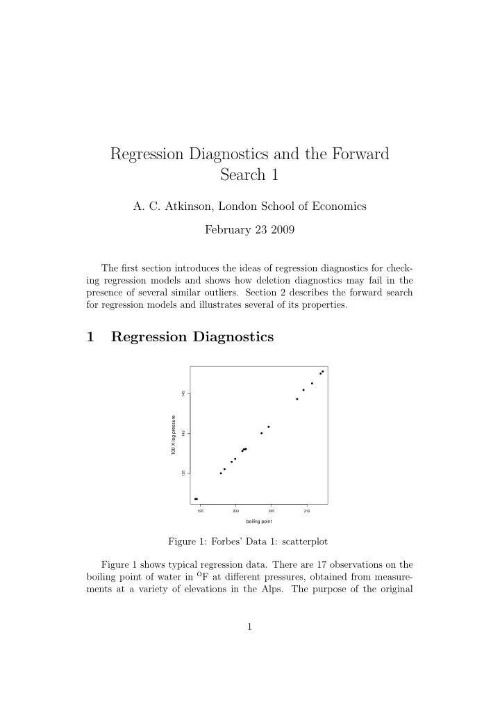
195 200 205 210 135 140 145

boiling point 100 X log pressure

Figure 1: Forbes’ Data 1: scatterplot Figure 1 shows typical regression data. There are 17 observations on the boiling point of water in oF at different pressures, obtained from measure- ments at a variety of elevations in the Alps. The purpose of the original 1

experiment was to allow prediction of pressure from boiling point, which is easily measured, and so to provide an estimate of altitude. Weisberg (1985) gives values of both pressure and 100 × log(pressure) as possible response. We consider only the latter, so that the variables are: x: boiling point, ◦F y: 100×log(pressure). Here there is one explanatory variable. Typically, in linear regression models, such as those used in the first chapter, there are n observations on a continuous response y. The expected value of the response E(Y ) is related to the values of p known constants by the relationship E(Y ) = Xβ. (1) Y is the n × 1 vector of responses, X is the n × p full-rank matrix of known constants and β is a vector of p unknown parameters. The model for the ith of the n observations can be written in several ways as, for example, yi = η(xi, β) + ǫi = xT

i β + ǫi = β0 + p−1

• j=1

βjxij + ǫi. (2) In the example η(xi, β) = β0 + β1xi. Under “second-order” assumptions the errors ǫi have zero mean, constant variance σ2 and are uncorrelated. That is, E(ǫi) = 0 and E(ǫiǫj) = σ2 i = j i = j . (3) Additionally we assume for regression that the errors are normally distrib- uted. Need to check:

• Whether any variables have been omitted;
• The form of the model;
• Are there unnecessary variables?
• Do the error assumptions hold

– Systematic departures: data transformation? – Isolated departures: outliers? 2

Plots of residuals are particularly important in checking models. The least squares estimates ˆ β minimize the sum of squares S(β) = (y − Xβ)T(y − Xβ) (4) and are ˆ β = (XTX)−1XTy, (5) a linear combination of the observations, which will be normally distributed if the observations are. These estimates have been found by minimizing the sum of squares S(β). The minimized value is the residual sum of squares S(ˆ β) = (y − X ˆ β)T(y − X ˆ β) = yTy − yTX(XTX)−1XTy = yT{In − X(XTX)−1XT}y, (6) where In is the n × n identity matrix, sometimes written I. The vector of n predictions from the fitted model is ˆ y = X ˆ β = X(XTX)−1XTy = Hy. (7) H is often called the hat matrix. Let the ith residual be ei = yi − ˆ yi, with the vector e = y − ˆ y = y − X ˆ β = (I − H)y. (8)

1.1 Residuals and Model Checking

Forbes’ Data 1. Insofar as the residuals ei estimate the unobserved errors ǫi there should be no relationship between ei and ˆ yi and the ei should be like a sample from a normal distribution. The LHP of Figure 2 is a plot of ei vs ˆ

• yi. The pattern appears random.

The RHP is a normal QQ plot of the ei. It would be straight if the residuals had exactly the values of order statistics from a normal distribution. Here the plot seems “pretty straight”. Can use simulation to obtain envelopes for the line. The conclusion is that model and data agree. Forbes’ Data 2. In fact, Forbes’ original data are as in Figure 3. Again a very straight line, but perhaps with an outlier near the centre of the range of x. The LHP of Figure 4 plots e against ˆ

• y. One observation (observation 12)

is clearly outlying. The QQ plot in the RHP is far from a straight line. How would we test whether observation 12 is outlying? 3

135 140 145 −0.2 −0.1 0.0 0.1

fitted values residuals

Quantiles of Standard Normal residuals −2 −1 1 2 −0.2 −0.1 0.0 0.1

Figure 2: Forbes’ Data 1: residuals against fitted values and Normal QQ plot

195 200 205 210 135 140 145

boiling point 100 X log pressure

Figure 3: Forbes’ Data 2: scatter plot. There appears to be a single slight

• utlier

4

135 140 145 0.0 0.5 1.0

fitted values residuals

Quantiles of Standard Normal residuals −2 −1 1 2 0.0 0.5 1.0

Figure 4: Forbes’ Data 2: residuals against fitted values and Normal QQ plot

1.2 Residuals and Leverage

Least squares residuals. e = (I − H)y so var e = (I − H)(I − H)Tσ2 = (I − H)σ2; the residuals do not all have the same variance. Estimate σ2 by s2 = S(ˆ β)/(n − p), where S(ˆ β) =

n

• i=1

e2

i = yT(I − H)y.

(9) Studentized residuals. With hi the ith diagonal element of H, var ei = (1 − hi)σ2. The studentized residuals ri = ei s

• (1 − hi)

= yi − ˆ yi s

• (1 − hi)

(10) have unit variance. However, they are not independent, nor do they follow a Student’s t distribution. That this is unlikely comes from supposing that ei is the only large residual, when s2 . = e2

i /(n − p), so that the maximum value

• f the squared studentized residual is bounded. Cook and Weisberg (1982,
• p. 19) show that r2

i /(n − p) has a beta distribution.

The quantity hi also occurs in the variance of the fitted values. From (7), var ˆ y = HHTσ2 = Hσ2, (11) 5

135 140 145 0.0 0.5 1.0

fitted values residuals

5 10 15 2 4 6 8 10 12

• bservation number

deletion residual

Figure 5: Forbes’ Data 2: residuals against fitted values (again) and deletion residuals against i so that the variance of ˆ yi = σ2hi. The value of hi is called the leverage of the ith observation. The average value of hi is p/n, with 0 ≤ hi ≤ 1. A large value indicates high leverage. Such observations have small l.s. residuals and high influence on the fitted model. Deletion Residuals. To test whether observation i is an outlier we compare it with an outlier free subset of the data, here the other n − 1

• bservations. Let ˆ

β(i) be the estimate of β when observation i is deleted. Then the deletion residual which tests for agreement of the observed and predicted values is r∗

i =

yi − xT

i ˆ

β(i) s(i)

• {1 + xT

i (XT (i)X(i))−1xi}

, (12) which, when the ith observation comes from the same population as the other

• bservations, has a t distribution on (n − p − 1) degrees of freedom. Results

from the Sherman–Morrison–Woodbury formula (Exercise) show that r∗

i =

ei s(i)

• (1 − hi)

= yi − ˆ yi s(i)

• (1 − hi)

. (13) There is no need to refit for each deletion. Forbes’ Data 2. Figure 5 compares the plot of ei against ˆ yi with that of r∗

i against ob-

servation number. The value for observation 12 is > 12. This is clearly an 6

135 140 145 −0.2 −0.1 0.0 0.1

fitted values residuals

5 10 15 −2 −1 1

• bservation number

deletion residual

Figure 6: Forbes’ Data 3 (observation 12 deleted): residuals against fitted values and deletion residuals against i

• utlier and should be deleted (better parameter estimates, tighter confidence

intervals, . . . ). Forbes’ Data 3. We delete observation 12. The LHP of Figure 6 shows ei against ˆ yi and the RHP the plot of r∗

i against observation number. There is

no further structure in either plot, so we accept that these 16 observations are all fitted by the linear model. Note that 2 deletion residuals have values < −2. What level should we test at? With n observations and an individual test of size α we will declare,

• n average nα outliers in a clean dataset. Use Bonferroni correction (level

α/n) to declare α% of datasets as containing outliers. Data with one leverage point. The LHP of Figure 7 shows data like Forbes’ data (no outlying observation 12) but with an extra observation at a point of higher leverage. The normal QQ plot of the RHP shows no dramatic departure from a straight line. Are the data homogeneous? We look at residuals. The LHP of Figure 8 plots ei against ˆ

• yi. There are

no particularly large residuals. But in the RHP observation 18 has a deletion residual around 4 - quite a significant value. But it might be foolish to delete the observation. Why? Backwards Elimination. These are examples of “backwards” analysis: find most extreme observation, delete it if outlying, reanalyse, check most extreme etc. Can fail due to “masking”: if there are several outliers, none 7

200 210 220 230 135 140 145 150 155 160 165

x y

Quantiles of Standard Normal residuals −2 −1 1 2 −0.3 −0.2 −0.1 0.0 0.1 0.2 0.3

Figure 7: Data with one leverage point: scatterplot and Normal QQ plot

135 140 145 150 155 160 165 −0.3 −0.2 −0.1 0.0 0.1 0.2 0.3

fitted values residuals

5 10 15 −2 −1 1 2 3 4

• bservation number

deletion residual

Figure 8: Data with one leverage point: residuals against fitted values and deletion residuals against i. RHP suggests there is a single outlier 8

Quantiles of Standard Normal residuals −2 −1 1 2 −4 −2 2 4 6 5 10 15 20 −1 1 2

• bservation number

deletion residual

Figure 9: Data with Four Leverage Points: Normal QQ plot of residuals and plot of deletion residuals against observation number may seem extreme. Data with Four Leverage Points. We now look at a simple example in which backward identification and elimination of outliers would fail. The LHP of Figure 9 shows the QQ plot of residuals for a set of 21

• bservations. Although there is some zig-zag patterning, there is no obvious

departure from linearity in the plot. The plot of deletion residuals against

• bservation number in the RHP seems completely without structure. There

appears therefore to be no evidence of the presence of outliers. The LHP of Figure 10 is a scatterplot of the data and shows that we have a straight line and a cluster of four points well off the line. The lot also shows the least squares line, which has been attracted towards the four leverage

• points. The plot of residuals against fitted values reveals the structure.

These plots are informative because they consider more than just the distribution of residuals. However, with several explanatory variables, such plots become harder to interpret. To detect outliers we need a “clean” part of the data against which to judge any other observations. In Figure 10 this would be the observations forming the linear pattern in the LHP. The four observations with high lever- age are remote from this line and would be revealed as outliers when judged against it. The forward search enables us to find outlier-free subsets of the data against which to judge potential outliers. 9

195 200 205 210 215 220 135 140 145

x y

136 138 140 142 144 −4 −2 2 4 6

fitted values residuals

Figure 10: Data with Four Leverage Points: scatterplot with least squares fit and residuals against fitted values

2 The Forward Search

2.1 General Principles

If the values of the parameters of the model were known, there would be no difficulty in detecting the outliers, which would have large residuals. The difficulty arises because the outliers are included in the data used to estimate the parameters, which can then be badly biased. Like most methods for

• utlier detection ours seeks to divide the data into two parts, a larger “clean”

part and the outliers. The clean data are then used for parameter estimation. The simplest example of this division of the data into two parts is in the use of single deletion diagnostics, such as those described above, where the division is into one potential outlier and the rest of the data. Standard books on regression diagnostics, such as Cook and Weisberg (1982), Atkinson (1985) and Chatterjee and Hadi (1988) include formulae for multiple deletion diagnostics, extending the results to consideration of a small number, perhaps two or three, of potential outliers at once. But the combinatorial explosion of the number of cases that have to be considered is a further severe drawback

• f such backwards working.

We use very robust methods to sort the data into a clean part and po- tential outliers. Our method starts from least median of squares (LMS). For the linear regression model E(Y ) = Xβ of (1), with X of rank p, let b be any estimate of β. With n observations the residuals from this estimate are ei(b) = yi − xT

i b, (i = 1, . . . , n). The LMS estimate ˆ

β∗

p is the value of b

10

minimizing the median of the squared residuals e2

i (b). Thus ˆ

β∗

p minimizes the

scale estimate σ2(b) = e2

[med](b),

(14) where e2

[k](b) is the kth ordered squared residual. In order to allow for esti-

mation of the parameters of the linear model the median is taken as med = [(n + p + 1)/2], (15) the integer part of (n + p + 1)/2. The very robust behaviour of the LMS estimate is in stark contrast to that of the least squares estimate ˆ β (5) minimizing (4). Only one outlier needs to be moved towards infinity to cause an arbitrarily large change in the estimate ˆ β: the breakdown point of ˆ β is zero. The LMS estimates at the beginning of the search can be very different from the least squares ones at the end, when outliers are present. We find an approximation to ˆ β∗

p by searching only over elemental sets,

that is, subsets of p observations, taken at random. We follow this proce-

• dure. Depending on the dimension of the problem we find the starting point

for the forward search either by sampling a few thousand subsets or by ex- haustively evaluating all subsets. We take as our initial subset that yielding the minimum value in (14), so obtaining an outlier free start for our forward search. In the forward search, larger subsamples of outlier free observations are found by starting from small subsets and incrementing them with observa- tions that have small residuals, and so are unlikely to be outliers. Suppose at some stage in the forward search the set of m observations used in fitting is S(m)

∗

. Fitting to this subset is by least squares (for regression models) yielding the parameter estimates ˆ β(m∗) . From these parameter estimates we can calculate a set of n residuals e(m∗) and we can also estimate σ2. Suppose that the subset S(m)

∗

is clear of outliers. There will then be n−m

• bservations not used in fitting that may contain outliers. Our interest is in

the evolution, as m goes from p to n, of quantities such as the residuals, parameter estimates and test statistics. In the absence of outliers and systematic departures from the model we expect both parameter estimates and residuals to remain sensibly constant during the forward search. We saw in the examples of Chapter 1 that this was so. If there are outliers, the forward procedure will include these towards the end of the search. Until these outliers are included, residual plots and parameter estimates will remain sensibly constant. 11

2.2 Step 1: Choice of the Initial Subset

If the model contains p parameters, our forward search algorithm for re- gression starts with the selection of a subset of p units. For the analysis of multivariate data we often start with m0 > p observations. Observations in this subset are intended to be outlier free.

2.3 Step 2: Adding Observations During the Forward Search

Given a subset of dimension m ≥ p, say S(m)

∗

, the parameters are found by least squares, giving the estimate ˆ β(m∗). We calculate the n residuals ei(m∗); the forward search moves to dimension m + 1 by selecting the m + 1 units with the smallest squared least squares residuals, the units being chosen by

• rdering all squared residuals e2

i (m∗), i = 1, . . . , n.

In most moves from m to m + 1 just one new unit joins the subset. It may also happen that two or more units join S(m+1)

∗

as one or more leave. This only occurs when the search includes one unit that belongs to a cluster

• f outliers. At the next step the remaining outliers in the cluster seem less
• utlying and so several may be included at once. Of course, several other

units then have to leave the subset.

2.4 Step 3: Monitoring the Search

Step 2 of the forward search is repeated until all units are included in the subset. If just one observation enters S(m)

∗

at each move, the algorithm provides an ordering of the data according to the specified null model, with

• bservations furthest from it joining the subset at the last stages of the

procedure. Remark 1: The estimate of σ2 does not remain constant during the for- ward search as observations are sequentially selected that have small residu-

• als. Thus, even in the absence of outliers, the residual mean square estimate

s2(m∗) < s2(n) = s2 for m < n. Important Plots.

• All n residuals at each step of the forward search. Large values of the

residuals among observations not in the subset indicate the presence of

• utliers.
• The residual sum of squares, or equivalently s2(m∗).

12

• For deletion of single observations Cook (1977) proposed the statistic

Di = (ˆ β(i) − ˆ β)TXTX(ˆ β(i) − ˆ β)/(ps2) (16) for detecting influential observations. Large values of Di indicate ob- servations that are influential on joint inferences about all the linear parameters in the model. We monitor a “forward version” of the Cook statistic Di. From the

• riginal definition in (16) this is given by

Dm = {ˆ β(m∗−1)−ˆ β(m∗)}TX(m∗)TX(m∗){ˆ β(m∗−1)−ˆ β(m∗)}/{ps2(m∗)}, (17) for m = p + 1, . . . , n, where X(m∗) is the m × p matrix that contains the m rows of the matrix X for the units in the subset.

• A further useful plot for outlier detection monitors the minimum dele-

tion residual among the units not belonging to the subset r∗

[m+1] = min |r∗ i (m∗)|

for i ∈ S(m)

∗

m = p + 1, . . . , n − 1. (18)

• An alternative is the maximum studentized residual in the subset

r[m] = max |ri(m∗)| for i ∈ S(m)

∗

m = p + 1, . . . , n. (19) Forbes’ Data 2. The plots showed a single outlier. It is not however clear whether this outlier is important. How does its presence change the inferences drawn from the data, such as the t test for regression, or the estimates of the parameters? Our forward method allows us to answer all such questions from a single search through the data. We start with a least squares fit to two robustly chosen observations. From this fit we calculate the residuals for all 17 observations and next fit to the three observations with smallest residuals etc. We expect that the last

• bservations to enter the search will be those which are furthest from the

model and so may cause changes once they are included in the subset used for fitting. Indeed observation 12 was the last to enter the search. For each value of m from 2 to 17 we calculate quantities such as the residuals and the parameter estimates and see how they change. Figure 11(a) is a plot of the values of the parameter estimates during the forward search. The values are extremely stable, reflecting the closeness of all observations to the straight line. The introduction of observation 12 at the end of the search causes virtually no change in the position of the line. However, Figure 11(b) 13

Subset size m Estimated beta coefficient 5 10 15

• 50
• 40
• 30
• 20
• 10

intercept slope

Subset size m s^2 5 10 15 0.0 0.05 0.10 0.15

Figure 11: Forbes’ data: parameter estimates from the forward search: (a) slope and intercept ˆ βo and ˆ β1 (the values are virtually unaffected by the outly- ing observation 12); (b) the value of the estimate of σ2 increases dramatically when observation 12 is included in the last step of the search

Subset size m Scaled residuals 5 10 15

• 1

1 2 3 4 5

12

Figure 12: Forbes’ data: forward plot of least squares residuals scaled by the final estimate of σ. Observation 12 is an outlier during the whole of this stable forward search 14

shows that introduction of observation 12 causes a huge increase in s2, the residual mean square estimate of the error variance σ2. The plots also imply that all other observations agree with the overall

• model. Figure 12 shows the residuals during the forward search. Throughout

the search, all observations have small residuals, apart from 12 which is

• utlying from all fitted subsets. Even when it is included in the last step of

the search, its residual only decreases slightly. Our analysis shows that Forbes’ data have a simple structure – there is

• ne outlying observation, 12, that is not influential for the estimates of the

parameters of the linear model. Inclusion of this observation does however cause the estimate s2 to increase from 0.0128 to 0.1436 with a corresponding decrease in the t statistic for regression from 180.73 to 54.45.

2.5 Hawkins’ Data

There are 128 observations and eight explanatory variables. The scatterplot matrix of the data in Figure 13 does not reveal an interpretable structure; there seems to be no relationship between y and seven of the eight explana- tory variables, the exception being x8. Some structure is however suggested by residual plots. The normal plot of least squares residuals in Figure 14(a) shows a cu- riously banded symmetrical pattern, with six apparent outliers. The data would seem not to be normal, but it is hard to know what interpretation to put on this structure. The normal plot of LMS residuals, Figure 14(b), shows (on counting) that 86 residuals are virtually zero, with three groups

• f almost symmetrical outliers from the model. Our forward search provides

a transition between these two figures. More helpfully, it enables us to mon- itor changes in residuals and parameter estimates and their significance as the apparent outliers are included in the subset used for fitting. Figure 15 is the forward plot of squared residuals, scaled by the final estimate of σ2. This shows three groups of residuals, the fourth group, the 86 smallest, being so small as to lie on the y axis of the plot. From m = 87

• nwards, the 24 observations with the next smallest residuals in Figure 14(b)

enter the subset. The growth in the subset causes changes in the other two groups of residuals; in particular, the most extreme observations become less

• so. After m = 110, the second group of outliers begins to enter the subset

and all residuals decrease. By the end of the process, the six largest outliers, cases 19, 21, 46, 73, 94 and 111 still form a distinct group, arguably more marked in Figure 15 than in Figure 14(a), which is a normal plot of the residuals when m = n. At the end of the search, the other groups of outliers are mixed together and masked. 15

X1

• 30

30

• 20

20

• 20

20 40 80

• 20

20

• 30

30

X2 X3

• 40

40

• 20

20

X4 X5

• 20

20

• 20

20

X6 X7

• 30

20 40 80

X8

• 20

20

• 40

40

• 20

20

• 30

20

• 10

5 15

• 10

5 15

y

Figure 13: Hawkins’ data: scatterplot matrix. The only apparent structure involving the response is the relationship between y and x8 16

Quantiles of standard normal LS residuals

• 2
• 1

1 2

• 10
• 5

5 10 Quantiles of standard normal LMS residuals

• 2
• 1

1 2

• 1000
• 500

500 1000

Figure 14: Hawkins’ data: normal plots of residuals. The least squares residuals in (a) seem to indicate six outliers and a nonnormal structure; there are 86 zero LMS residuals in (b)

Subset size m Scaled squared residuals 20 40 60 80 100 120 5 10 15

19 21 46 73 94 111

Figure 15: Hawkins’ data: forward plot of scaled squared residuals. The three groups of outliers are clearly shown, as is the effect of masking of some

• utliers at the end of the search

17

• Max. studentized residual

20 40 60 80 100 120 2 4 6 8 10 Subset size m

• Min. deletion residual

20 40 60 80 100 120 5 10 15 20

Figure 16: Hawkins’ data: forward plot of (a) the maximum studentized residual in the subset used for fitting (19) and (b) the minimum deletion residual outside the subset (18). The effects of the three groups of outliers are evident Several other plots also serve to show that there are three groups of

• utliers. Three are similar in appearance.

The Cook distances (not shown here) reflect changes in parameter esti- mates as the forward search progresses and show three peaks due to the large changes from the initial inclusion of each group of observations. Figures 16(a) and (b) show similar patterns, but in plots of the residuals. Figure 16(a) shows the maximum studentized residual in the subset used for fitting (19). This will be large when one or two outliers are included in the subset. Fi- nally in this group of three plots, Figure 16(b) shows the minimum deletion residual at each stage (18), where the minimization is over those cases not yet in the subset. The three peaks in the figure show the distance of the nearest observation from the model that has been fitted so far. The first peak is the largest because the variance of the first 86 cases is so small. The declining shape of each peak is caused by the increase in s2 as outliers are introduced during the search, which reduces the size of the deletion residuals. At the end of the peaks there is nothing remarkable about the values of the deletion residuals. In this example the two plots of the residuals and that of the modified Cook distances are very similar in structure. In other examples, not only may the plot of the Cook distances be different from that of the 18

Predicted values Residuals

• 500

500 1500

• 500

500 1000 Quantiles of standard normal Studentized residuals

• 2
• 1

1 2

• 2
• 1

1 2 3

Figure 17: Wool data: (a) least squares residuals e against fitted values ˆ y; (b) normal QQ plot of studentized residuals residual plots, but the two residual plots may also be distinct. These plots are one way in which the forward search reveals the masked nature of the

• utliers. Another is from forward residual plots such as Figure 15.

The clear nature of the outlier structure of these data is in sharp contrast to that of some other examples.

2.6 Wool Data

In this example we show the effect of the ordering of the data during the for- ward search on the estimates of regression coefficients and the error variance The data, taken from Box and Cox (1964), give the number of cycles to failure of a worsted yarn under cycles of repeated loading. The results are from a single 33 factorial experiment. In their analysis Box and Cox (1964) recommend that the data be fitted after the log transformation of y. We analyse the untransformed data, to show the information provided by the forward search. Figure 17(a) is a plot of residuals against fitted values when a first-order model in the three factors is fitted to the data. It has a curved shape with increasing variability at the right-hand end of the plot, typical evidence of the need for a transformation. Similar evidence is provided by the normal plot of residuals in Figure 17(b). Here the curved shape is a reflection of the 19

Subset size m Scaled residuals 5 10 15 20 25

• 2

2 4 6 19 20 21 22 10 9

Figure 18: Wool data: forward plot of least squares residuals scaled by the final estimate of σ. The three largest residuals can be directly related to the levels of the factors skewed distribution of the residuals. To investigate the impact of individual

• bservations on the fit, we turn to the forward search.

The forward plot of residuals is in Figure 18; in this plot we give the scaled residuals themselves, rather than the squared values. It is typical of such plots that the residuals in the early stages are far from symmetrical;

• nly the residuals of the m observations in the subset are constrained to sum

to zero. For most of the search the four largest residuals are for observations 19, 20, 21 and 22. Since the data are in standard order for a three-level factorial, these consecutive case numbers suggest some systematic failure of the model. In fact these are the four largest observations, arising when the first factor is at its highest level and, for the three largest, the second factor is at its lowest. Such extreme observations are likely to provide evidence for a transformation. Other forward plots indicate the way in which the model changes as more

• bservations are introduced.

The value of R2, Figure 19(a), decreases to around 0.8 for part of the search, with a final value of 0.729. Further evidence

• f a relationship that changes with the search is given by the forward plot
• f estimated coefficients in Figure 19(b). Initially the values are stable, but

20

Subset size m R^2 5 10 15 20 25 0.70 0.80 0.90 1.00 Subset size m Estimated beta coefficient 5 10 15 20 25

• 500

500 1000

beta_0 beta_1 beta_2 beta_3

Figure 19: Wool data: (a) the multiple correlation coefficient R2 during the forward search and (b) the values of the parameter estimates later they start to diverge.

• Envelopes. An important aspect of the interpretation of such plots is

the provision of simulation (or other) envelopes to calibrate what departures are expected to be present. Riani and Atkinson (2007) provide envelopes for outliers in regression when the statistic is the minimum deletion residual amongst those not in the subset. Further details on the FS in regression are in Chapters 1 to 3 of Atkinson and Riani (2000)

2.7 Exercises

• 1. Expressions for the effect of deletion are based on a matrix relationship
• ften called the Sherman–Morrison–Woodbury formula.

Let A be a square p×p matrix and let U and V be matrices of dimension p × m. Verify that (A − UV T)−1 = A−1 + A−1U(Im − V TA−1U)−1V TA−1, (20) where it is assumed that all necessary inverses exist.

• 2. For regression we let A = XTX. The ith row of X is xT

i . Deletion of

21

this row leaves the matrix X(i). With this definition XT

(i)X(i) = (XTX − xixT i ).

Find an expression for (XT

(i)X(i))−1 that depends on the old inverse (XTX)−1,

• n xi and on the leverage measure hi.
• 3. Hence find ˆ

β(i) and (n − p − 1)s2

(i). So derive (13).

• 4. Consider data like that in Figure 10. Fit a straight line to the data

following the linear relationship. Then successively add one of the points from the cluster on the right. Monitor what happens to the residuals, the parameter estimates and the fitted line. What happens if a backwards outlier rejection procedure is used in the RHP of the figure?

References

Atkinson, A. C. (1985). Plots, Transformations, and Regression. Oxford: Oxford University Press. Atkinson, A. C. and M. Riani (2000). Robust Diagnostic Regression Analy-

• sis. New York: Springer–Verlag.

Box, G. E. P. and D. R. Cox (1964). An analysis of transformations (with discussion). Journal of the Royal Statistical Society, Series B 26, 211– 246. Chatterjee, S. and A. S. Hadi (1988). Sensitivity Analysis in Linear Re-

• gression. New York: Wiley.

Cook, R. D. (1977). Detection of influential observations in linear regres-

• sion. Technometrics 19, 15–18.

Cook, R. D. and S. Weisberg (1982). Residuals and Influence in Regression. London: Chapman and Hall. Riani, M. and A. C. Atkinson (2007). Fast calibrations of the forward search for testing multiple outliers in regression. Advances in Data Analysis and Classification, 123–141. doi:10.1007/s11634-007-0007-y. Weisberg, S. (1985). Applied Linear Regression (2nd edition). New York: Wiley. 22