refresh counting cs70 on to probability key points
play

Refresh: Counting. CS70: On to probability. Key Points First Rule - PowerPoint PPT Presentation

Refresh: Counting. CS70: On to probability. Key Points First Rule of counting: Objects from a sequence of choices: n i possibilitities for i th choice. Uncertainty does not mean nothing is known Modeling Uncertainty: Probability Space


  1. Refresh: Counting. CS70: On to probability. Key Points First Rule of counting: Objects from a sequence of choices: n i possibilitities for i th choice. ◮ Uncertainty does not mean “nothing is known” Modeling Uncertainty: Probability Space n 1 × n 2 ×···× n k objects. ◮ How to best make decisions under uncertainty? Second Rule of counting: If order does not matter. ◮ Buy stocks Count with order. Divide by number of orderings/sorted object. 1. Key Points � n � ◮ Detect signals (transmitted bits, speech, images, radar, Typically: . k 2. Random Experiments diseases, etc.) Stars and Bars: Sample k objects with replacement from n . ◮ Control systems (Internet, airplane, robots, self-driving � n + k − 1 Order doesn’t matter. k stars n − 1 bars. Typically: � or 3. Probability Space k cars, schedule surgeries in a hospital, etc.) � n + k − 1 � . n − 1 ◮ How to best use ‘artificial’ uncertainty? Inclusion/Exclusion: two sets of objects. Add number of each and then subtract intersection of sets. ◮ Play games of chance Sum Rule: If disjoint just add. ◮ Design randomized algorithms. Combinatorial Proofs: Identity from counting same in two ways. � n ◮ Probability � n + 1 � n � � � Pascal’s Triangle Example: = + . k k − 1 k ◮ Models knowledge about uncertainty RHS: Number of subsets of n + 1 items size k . � n � ◮ Optimizes use of knowledge to make decisions LHS: counts subsets of n + 1 items with first item. k − 1 � n � counts subsets of n + 1 items without first item. k Disjoint – so add! The Magic of Probability Random Experiment: Flip one Fair Coin Random Experiment: Flip one Fair Coin Flip a fair coin: Uncertainty: vague, fuzzy, confusing, scary, hard to think about. Probability: A precise, unambiguous, simple(!) way to think about Flip a fair coin: ( One flips or tosses a coin ) uncertainty. What do we mean by the likelihood of tails is 50 % ? Two interpretations: ◮ Single coin flip: 50% chance of ‘tails’ [subjectivist] ◮ Possible outcomes: Heads ( H ) and Tails ( T ) Willingness to bet on the outcome of a single flip ( One flip yields either ‘heads’ or ‘tails’. ) ◮ Many coin flips: About half yield ‘tails’ [frequentist] ◮ Likelihoods: H : 50 % and T : 50 % Our mission: help you discover the serenity of Probability, i.e., enable Makes sense for many flips you to think clearly about uncertainty. ◮ Question: Why does the fraction of tails converge to the same Your cost: focused attention and practice on examples and problems. value every time? Statistical Regularity! Deep!
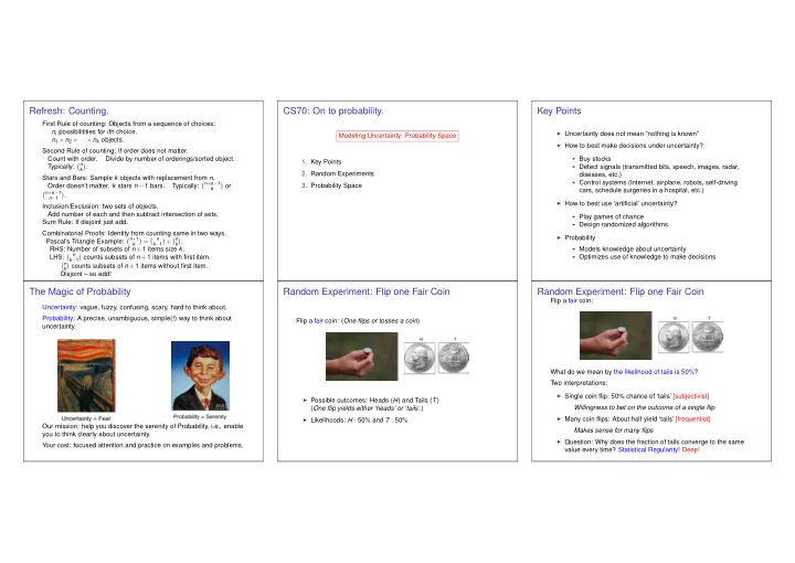
  2. T H Random Experiment: Flip one Fair Coin Random Experiment: Flip one Unfair Coin Random Experiment: Flip one Unfair Coin Flip a fair coin: model Flip an unfair (biased, loaded) coin: Flip an unfair (biased, loaded) coin: model Ω p ◮ Possible outcomes: Heads ( H ) and Tails ( T ) ◮ Likelihoods: H : p ∈ ( 0 , 1 ) and T : 1 − p 1 - p ◮ The physical experiment is complex. (Shape, density, initial ◮ Frequentist Interpretation: Physical Experiment Probability Model momentum and position, ...) Flip many times ⇒ Fraction 1 − p of tails ◮ The Probability model is simple: ◮ Question: How can one figure out p ? Flip many times ◮ A set Ω of outcomes: Ω = { H , T } . ◮ Tautology? No: Statistical regularity! ◮ A probability assigned to each outcome: Pr [ H ] = 0 . 5 , Pr [ T ] = 0 . 5. Flip Two Fair Coins Flip Glued Coins Flip two Attached Coins Flips two coins attached by a spring: Flips two coins glued together side by side: ◮ Possible outcomes: { HH , HT , TH , TT } ≡ { H , T } 2 . ◮ Note: A × B := { ( a , b ) | a ∈ A , b ∈ B } and A 2 := A × A . ◮ Likelihoods: 1 / 4 each. ◮ Possible outcomes: { HT , TH } . ◮ Possible outcomes: { HH , HT , TH , TT } . ◮ Likelihoods: HH : 0 . 4 , HT : 0 . 1 , TH : 0 . 1 , TT : 0 . 4. ◮ Likelihoods: HT : 0 . 5 , TH : 0 . 5. ◮ Note: Coins are glued so that they show different faces. ◮ Note: Coins are attached so that they tend to show the same face, unless the spring twists enough.

  3. Flipping Two Coins Flipping Two Coins Flipping n times Flip a fair coin n times (some n ≥ 1): Here is a way to summarize the four random experiments: ◮ Possible outcomes: { TT ··· T , TT ··· H ,..., HH ··· H } . Thus, 2 n possible outcomes. ◮ Note: { TT ··· T , TT ··· H ,..., HH ··· H } = { H , T } n . A n := { ( a 1 ,..., a n ) | a 1 ∈ A ,..., a n ∈ A } . | A n | = | A | n . ◮ Likelihoods: 1 / 2 n each. Important remarks: ◮ Each outcome describes the two coins. ◮ E.g., HT is one outcome of each of the above experiments. ◮ Ω is the set of possible outcomes; ◮ It is wrong to think that the outcomes are { H , T } and that one ◮ Each outcome has a probability (likelihood); picks twice from that set. ◮ The probabilities are ≥ 0 and add up to 1; ◮ Indeed, this viewpoint misses the relationship between the two ◮ Fair coins: [ 1 ] ; Glued coins: [ 3 ] , [ 4 ] ; flips. Spring-attached coins: [ 2 ] ; ◮ Each ω ∈ Ω describes one outcome of the complete experiment. ◮ Ω and the probabilities specify the random experiment. Roll two Dice Probability Space. Probability Space: formalism. Ω is the sample space. Roll a balanced 6-sided die twice: 1. A “random experiment”: ω ∈ Ω is a sample point . (Also called an outcome .) ◮ Possible outcomes: { 1 , 2 , 3 , 4 , 5 , 6 } 2 = { ( a , b ) | 1 ≤ a , b ≤ 6 } . (a) Flip a biased coin; Sample point ω has a probability Pr [ ω ] where (b) Flip two fair coins; ◮ Likelihoods: 1 / 36 for each. ◮ 0 ≤ Pr [ ω ] ≤ 1; (c) Deal a poker hand. ◮ ∑ ω ∈ Ω Pr [ ω ] = 1 . 2. A set of possible outcomes: Ω . (a) Ω = { H , T } ; (b) Ω = { HH , HT , TH , TT } ; | Ω | = 4; (c) Ω = { A ♠ A ♦ A ♣ A ♥ K ♠ , A ♠ A ♦ A ♣ A ♥ Q ♠ ,... } � 52 | Ω | = � . 5 3. Assign a probability to each outcome: Pr : Ω → [ 0 , 1 ] . (a) Pr [ H ] = p , Pr [ T ] = 1 − p for some p ∈ [ 0 , 1 ] (b) Pr [ HH ] = Pr [ HT ] = Pr [ TH ] = Pr [ TT ] = 1 4 � 52 (c) Pr [ A ♠ A ♦ A ♣ A ♥ K ♠ ] = ··· = 1 / � 5

  4. ω ω Probability Space: Formalism. Probability Space: Formalism Probability Space: Formalism Simplest physical model of a uniform probability space: Simplest physical model of a non-uniform probability space: In a uniform probability space each outcome ω is equally probable: 1 Pr [ ω ] = | Ω | for all ω ∈ Ω . Ω Ω P r [ ω ] P r [ ω ] 1/8 Red 3/10 Red Green 1/8 . Green 4/10 ... . . Yellow 2/10 Maroon 1/8 Blue 1/10 Probability model Physical experiment Physical experiment Probability model Examples: A bag of identical balls, except for their color (or a label). If the bag is ◮ Flipping two fair coins, dealing a poker hand are uniform Ω = { Red, Green, Yellow, Blue } well shaken, every ball is equally likely to be picked. probability spaces. Pr [ Red ] = 3 10 , Pr [ Green ] = 4 10 , etc. Ω = { white, red, yellow, grey, purple, blue, maroon, green } ◮ Flipping a biased coin is not a uniform probability space. Pr [ blue ] = 1 8 . Note: Probabilities are restricted to rational numbers: N k N . Probability Space: Formalism An important remark Summary of Probability Basics Physical model of a general non-uniform probability space: Modeling Uncertainty: Probability Space Ω ◮ The random experiment selects one and only one outcome in Ω . p ω P r [ ω ] ◮ For instance, when we flip a fair coin twice 1. Random Experiment p 1 p 3 Green = 1 ◮ Ω = { HH , TH , HT , TT } 3 2. Probability Space: Ω; Pr [ ω ] ∈ [ 0 , 1 ]; ∑ ω Pr [ ω ] = 1. p 2 ◮ The experiment selects one of the elements of Ω . Purple = 2 ... . . . 3. Uniform Probability Space: Pr [ ω ] = 1 / | Ω | for all ω ∈ Ω . 1 2 ◮ In this case, its wrong to think that Ω = { H , T } and that the Yellow p ω experiment selects two outcomes. p 2 ◮ Why? Because this would not describe how the two coin flips Fraction p 1 of circumference are related to each other. Physical experiment Probability model ◮ For instance, say we glue the coins side-by-side so that they face up the same way. Then one gets HH or TT with probability The roulette wheel stops in sector ω with probability p ω . 50 % each. This is not captured by ‘picking two outcomes.’ Ω = { 1 , 2 , 3 ,..., N } , Pr [ ω ] = p ω .

Download Presentation
Download Policy: The content available on the website is offered to you 'AS IS' for your personal information and use only. It cannot be commercialized, licensed, or distributed on other websites without prior consent from the author. To download a presentation, simply click this link. If you encounter any difficulties during the download process, it's possible that the publisher has removed the file from their server.

Recommend


More recommend