Recently I had to review a paper, where a CNN was used Visualizing - - PDF document

Visualizing Crash Data Patterns

Peter Wagner, with Ragna Hoffmann, Marek Junghans, Andreas Leich, and Hagen Saul German Aerospace Center (DLR) – Institute of Transport Systems 32nd ICTCT Conference 2019 Warsaw, Poland 25 October 2019

Recently…

• I had to review a paper, where a CNN was used

to predict crashes online (their probability)

• Not all reviewers were happy with this paper, therefore an interesting discussion

between reviewers and editor started

• One reviewer deems this impossible to work, since CNN’s search for patterns:
• I hope that anybody agrees with me, that this reviewer is wrong

However, crashes are essentially rare events and many are pure random (e.g. due to drunk drivers, drunk pedestrians) with no pattern at all.

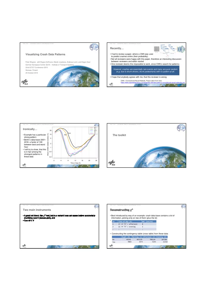
CNN = Convolutional Neural Network, Picture taken from here: https://www.superdatascience.com/blogs/the-ultimate-guide-to-convolutional-neural-networks-cnn 0.2 0.5 1 2 5 10 20 Time of day (h) Share of BAC-related crashes (%) Sun

Sat 4 8 12 16 20 24

Ironically…

• Example has a particular

strong pattern

• Berlin’s data-base 2001–

2016: a factor of 100 between best and worst hour

• I will try to show, that this

is in fact among the strongest patterns in these data

The toolkit

Two main instruments

• Best introduced by way of an example: crash data-base contains a lot of

information, picking only on two of them (plus the id):

• Constructing the contingency table (cross table) from these data

Id Time-of-day (h) BAC (yes/no) 1 17 “2” / afternoon 2 22 “3” / evening 1 … … … Night (0) Morning (1) Afternoon (2) Evening (3) No 49343 497179 705124 287286 Yes 9843 3573 5193 11316

Dependencies

Night Morning Afternoon Evening Sum No 49343 497179 705124 287286 1538932 Yes 9843 3573 5193 11316 29925 Sum 59186 500752 710317 298602

Yielding…

Night Morning Afternoon Evening No

• 36.2

8.5 10.0

• 10.4

Yes 259.3

• 61.2
• 71.8

74.5

A few side remarks

• 72
• 4

260 Pearson residuals: p-value < 2.22e-16 ToD BAC Night 1 Morning Afternoon Evening

Data and Results

A glimpse into the data-set

• Data-set in its original form has ~60 variables
• Added another ~60 or so, such as weather, demand (DTV – model-based),…
• Apart from a fairly precise geo-location, data contain the collision diagram
• From these sets, the following variables have been picked:
• year, hour, weekDay,
• crash-type (cType), vehicle type (vType), collision diagram (colDia)
• nAll, nFatal, nHeavy, nLight,
• BAC, age, sex,
• adt2009, temp, humidity
• Tried not to aggregate, but e.g. for age, adt, temp, humidity we had to

Collision diagrams

• Data contain collision

diagrams for each crash

• Pick the 12 most likely

collision diagrams in the following

• Lines of data:
• Original:

3.17M

• Crashes:

1.57M

• 12 most:

1.07M

Then, brute-force

The Top 10 (BAC/ hour is in it!)

Var1 Var2 rank avCV avRank sdRank Comment cType colDia 1 0,7492 1 Trivial cType vType 2 0,3996 2 Trivial? sex vType 3 0,2424 3,2 0,42 Interesting hour BAC 4 0,2252 4,1 0,57 As promised age vType 5 0,1969 5,3 0,48 colDia vType 6 0,1911 6,3 0,48 temp humidity 7 0,1696 7,3 0,48 Not surprising cType age 8 0,1572 8,4 0,70 nHeavy vType 11 0,1465 9,7 1,25 cType adt2009 9 0,1441 10,6 0,70

Looking closer… (4th rank) – V = 0.23

• 25
• 4

2 95 Pearson residuals: p-value = < 2.22e-16 hour BAC 1 1 2 3 4 5 6 7 8 9 10 11 12 13 14 15 16 17 18 19 20212223

Looking closer… (1st rank) V = 0.749

• 270
• 4

890 Pearson residuals: p-value = < 2.22e-16 colDia cType 11 7 6 5 4 3 2 1 17 48 49 50 56 58 61 70 75 84 111

A weak one, rank 111, V = 0.01 … many more

• 4.9
• 4.0
• 2.0

Rank 37 – V = 0.05 … many more

• 37
• 4

4 33 Pearson residuals: p-value = < 2.22e-16 year age 2001 (61,107] (52,61] (46,52] (40,46] (35,40] (29,35] (24,29] (17,24] (0,17] 2002 2003 2004 2005 2006 2007 2008 2009 2010 2011 2012 2013 2014 2015 2016

Conclusions

• We have investigated a rarely used tool to analyze a crash data-base
• It clearly needs a huge amount of crashes to work
• For these, then, it produces a very general kind of “correlation” between each two

variables that have been recorded and may or may not have a causal connection

• They can be sorted according to Cramér’s V (or any other similar measure) to find

the ones with a large correlation

• These interesting ones of these are to be analyzed by a mosaic plot
• It gives a huge amount of information…
• Question to all: is this interesting? What of this is interesting?

Thank you for listening. Any questions?

Peter Wagner Deutsches Zentrum für Luft- und Raumfahrt e.V. (DLR) German Aerospace Center | Institute of Transportation Systems Rutherfordstrasse 2 | 12489 Berlin | Germany +49 30 67055-237 | peter.wagner@dlr.de | DLR.de/ts

Yielding…

Night Morning Afternoon Evening No

• 36.2

8.5 10.0

• 10.4

Yes 259.3

• 61.2
• 71.8

74.5

Collision diagrams

• Make the share

variable violin plots…

• Can be done by

subdividing the data,

• r by

Robustness of the rank

• Plotted against the rank

in the full data-set

A glimpse into the data-set

• Data-set in its original form has ~60 variables
• Added another ~60 or so, such as weather, demand (DTV – model-based),…
• We may use the information from the German travel demand surveys in addition,

to get a distribution of the traffic over time-of-day, mode, and the like

• Apart from a fairly precise geo-location, data contain the collision diagram
• From these sets, the following variables have been picked:
• year, hour, weekDay,
• streetCat, crash-type (cType), vType, collision diagram (colDia)
• nAll", "nFatal", "nHeavy", "nLight",
• "BAC", "age", "sex",
• "adt2009", "temp", "humidity"

Looking closer… (2nd rank) … too complex – V = 0.4

• 150
• 4

850 Pearson residuals: p-value = < 2.22e-16 vType cType 1 7 6 5 4 3 2 1 234 11 12 13 15 20 21 = car 22 31 32 33 34 35 40 41 42 43 44 45 46 48 51 52 53 54 55 57 58 59 61 71 72 81 82 83 84 919293

Looking closer… (3rd rank) – V = 0.24

• 140
• 4

88 Pearson residuals: p-value = < 2.22e-16 vType sex 1 F M 23 4 112 13 15 20 21 = car 22 31 32 334 35 40 41 42 43 44 45 46 48 51 52 53 54 55 57 58 59 61 71 72 81 82 83 84 91 92 93

This is rank 8

• 65
• 4

350 Pearson residuals: p-value = < 2.22e-16 age cType (0,17] 7=Misc 6=rear-end 5=with parking 4=ped crossing 3 2 = turning 1 (17,24] (24,29] (29,35] (35,40] (40,46] (46,52] (52,61] (61,107]

Rank 20, V = 0.083

• 54
• 4

4 130 Pearson residuals: p-value = < 2.22e-16 colDia age 11 (61,107] (52,61] (46,52] (40,46] (35,40] (29,35] (24,29] (17,24] (0,17] 17 48 49 50 56 58 61 70 75 84 111