Recap: VINCIA Plug-in to PYTHIA 8 C++ (~20,000 lines) Giele, - PowerPoint PPT Presentation

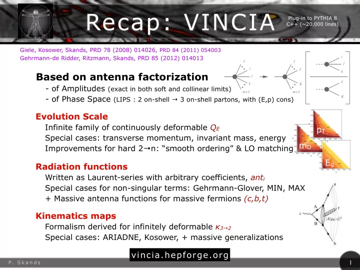
Recap: VINCIA Plug-in to PYTHIA 8 C++ (~20,000 lines) Giele, Kosower, Skands, PRD 78 (2008) 014026, PRD 84 (2011) 054003 Gehrmann-de Ridder, Ritzmann, Skands, PRD 85 (2012) 014013 i 1 1 j i I k Based on antenna factorization j I k K - of Amplitudes (exact in both soft and collinear limits) m+1 m+1 - of Phase Space (LIPS : 2 on-shell → 3 on-shell partons, with (E,p) cons) K 1.0 Evolution Scale 0.6 0.8 0.6 Infinite family of continuously deformable Q E y jk 1.0 p T 0.4 0.8 0.2 0.8 0.2 0.2 Special cases: transverse momentum, invariant mass, energy ⌦ ↵ 0.4 0.6 0.8 0.4 0.0 y jk 0.0 0.2 0.4 0.6 0.8 1.0 m D 0.4 0.8 1.0 y ij 0.6 0.6 Improvements for hard 2 → n: “smooth ordering” & LO matching 0.8 0.2 0.4 0.2 0.6 0.0 0.0 0.2 0.4 0.6 0.8 1.0 y jk y ij 0.4 E g 0.6 Radiation functions 0.2 0.2 0.8 0.0 0.4 0.0 0.2 0.4 0.6 0.8 1.0 y ij Written as Laurent-series with arbitrary coefficients, ant i ∗ √ 2 (c) Special cases for non-singular terms: Gehrmann-Glover, MIN, MAX + Massive antenna functions for massive fermions (c,b,t) Kinematics maps Formalism derived for infinitely deformable κ 3 → 2 Special cases: ARIADNE, Kosower, + massive generalizations vincia.hepforge.org 1 P. S k a n d s

One-Loop Corrections Giele, Kosower, Skands, Phys.Rev. D78 (2008) 014026 Trivial Example (for notation) : Z → qq First Order (~POWHEG) Z 0 → q ¯ q Fixed Order: Exclusive 2-jet rate (2 and only 2 jets), at Q = Q had Z Q 2 ! 1 + 2 Re[ M 0 0 M 1 ∗ ] had ∗ ] = | M 0 0 | 2 0 d Φ ant g 2 + s C A g/q ¯ q | M 0 0 | 2 q = | M 0 1 | 2 0 Born Virtual Unresolved Real ¯ | M 0 0 | 2 Markov Shower: Exclusive 2-jet rate (2 and only 2 jets), at Q = Q had Z s ! 0 | 2 ∆ ( s, Q 2 | M 0 had ) = | M 0 0 | 2 d Φ ant g 2 q + O ( α 2 1 − s C A g/q ¯ s ) Q 2 had Born Sudakov Approximate Virtual + Unresolved Real NLO Correction: Subtract and correct by difference 2 Re[ M 0 0 M 1 ∗ ] ) = ↵ s 0 q ( ✏ , µ 2 /m 2 � � 2 ⇡ 2 C F 2 I q ¯ Z ) − 4 | M 0 0 | 2 ⇣ 1 + α s ⌘ 0 | 2 → | M 0 | M 0 0 | 2 Z s ✓ ◆ Z ) + 19 π q = ↵ s d Φ ant 2 C F g 2 q ( ✏ , µ 2 /m 2 s A g/q ¯ 2 ⇡ 2 C F − 2 I q ¯ 4 0 IR Singularity Operator 2 P. S k a n d s

One-Loop Corrections Ongoing work, with E. Laenen & L. Hartgring (NIKHEF) Getting Serious: second order Fixed Order: Exclusive 3-jet rate (3 and only 3 jets), at Q = Q had Z Q 2 d Φ 2 had 1 | 2 + 2 Re[ M 0 Exact → | M 0 1 M 1 ∗ | M 0 2 | 2 1 ] + d Φ 1 0 Born Virtual Unresolved Real Markov Shower: d σ q ¯ q m Z 2 → 3 Evolution q ( m 2 Z , Q 2 E ) ∆ q ¯ Q E a g/q ¯ q Q R 3 → 4 Evolution ∆ qg ( Q 2 q ( Q 2 R , 0) ∆ g ¯ R , 0) 0 1 | 2 ∆ 2 ( m 2 Approximate → (1 + V 0 ) | M 0 Z , Q 2 1 ) ∆ 3 ( Q 2 R 1 , Q 2 had ) , V 0 = α s / π 2 → 3 Evolution 3 → 4 Evolution µ R 3 P. S k a n d s

Master Equation Ongoing work, with E. Laenen & L. Hartgring (NIKHEF) NLO Correction: Subtract and correct by difference A NLO = A LO (1+V 1 ) V 0 µ R � LC  2 Re[ M 0 1 M 1 ⇤ ✓ µ 2 1 ] ✓ 11 N C − 2 n F ◆ ◆ − ↵ s − ↵ s ME V 1 Z ( q, g, ¯ q ) = ln | M 0 µ 2 1 | 2 2 ⇡ 6 ⇡ PS " # Gluon Emission IR + ↵ s C A q ) + 34 Standard IR − 2 I (1) qg ( ✏ , µ 2 /s qg ) − 2 I (1) qg ( ✏ , µ 2 /s g ¯ Singularity Singularities 2 ⇡ 3 Standard " # + ↵ s n F Gluon Splitting IR − 2 I (1) qg,F ( ✏ , µ 2 /s qg ) − 2 I (1) Finite Terms q,F ( ✏ , µ 2 /s qg ) − 1 Singularity g ¯ 2 ⇡ δ A = LO Matching Z m 2 Z m 2 " + ↵ s C A Z Z Terms (finite) 8 ⇡ 2 d Φ ant A std q + 8 ⇡ 2 2 → 3 Sudakov Logs d Φ ant � A g/q ¯ q g/q ¯ 2 ⇡ Q 2 Q 2 δ A 2 → 3 Q 1 = 3-parton 1 1 Resolution Scale Z s j Z s j 2 2 # X X 8 ⇡ 2 d Φ ant (1 − O Ej ) A std 8 ⇡ 2 g/qg + d Φ ant � A g/qg 3 → 4 Emit − 0 0 O Ej = Gluon-Emission δ A 3 → 4, Emit j =1 j =1 Ordering Function 3 → 4 Z s j Z s j 2 2 " + ↵ s n F Sudakov X 8 ⇡ 2 d Φ ant (1 − O Sj ) P Aj A std X 8 ⇡ 2 q/qg + d Φ ant � A ¯ − q/qg Logs ¯ 2 ⇡ 0 0 δ A 3 → 4, Split O Sj = Gluon-Splitting j =1 j =1 Ordering Function 3 → 4 Split ◆ # − 1 s qg − s g ¯ ✓ s qg q ln , (72) 6 s qg + s g ¯ s g ¯ q q *) Note: here only Leading Color 4 P. S k a n d s

Loop Corrections Ongoing work, with E. Laenen & L. Hartgring (NIKHEF) (MC) 2 : NLO Z → 2 → 3 Jets + Markov Shower Q E = 2 p T H strong L Size of NLO 0 1.75 1.5 Correction: Quark-Collinear 1.4 Hard over 3-parton Resolved g ( p j ) Phase Space - 2 1.5 q ( p k ) ¯ Markov 1.5 Evolution in: ln H y jk L Transverse - 4 2 Momentum q ( p i ) 1.75 Parameters: - 6 Scaled Invariants α S (M Z ) = 0.12 1.75 µ R = m Z y ij = ( p i · p j ) Λ QCD = Λ MS Soft Antiquark-Collinear M 2 Z - 8 → 0 when i||j - 8 - 6 - 4 - 2 0 & when E j → 0 ln H y ij L 5 P. S k a n d s

Choice of µ R Ongoing work, with E. Laenen & L. Hartgring (NIKHEF) A) M Z B) p T “Typical” Fixed-Order Choice = “Typical” Shower Choice Q E = 2 p T H strong L Q E = 2 p T H strong L 0 0 1.75 1.5 1.2 1.2 1.4 1.2 1.1 µ R = m Z µ R = p Tg - 2 - 2 1.5 1.1 Λ QCD = Λ CMW 1.5 Λ QCD = Λ MS 1.2 ln H y jk L ln H y jk L - 4 - 4 1.05 2 1.75 - 6 - 6 1.75 1.1 - 8 - 8 - 8 - 6 - 4 - 2 0 - 8 - 6 - 4 - 2 0 ln H y ij L ln H y ij L Markov Evolution in: Transverse Momentum, α S (M Z ) = 0.12 6 P. S k a n d s

Choice of Q Evol Ongoing work, with E. Laenen & L. Hartgring (NIKHEF) Q E = m D Q E = 2 p T H strong L 0 2 1.75 1.3 0 1.5 1.2 1.2 1.2 1.2 1.1 1.1 1.4 1.05 - 2 - 2 1.2 Markov Evolution in Markov Evolution 1.1 0.95 1.2 0.9 m D2 = 2min(s ij ,s jk ) in p TA2 = s ij s jk /s ijk ln H y jk L 1.3 ln H y jk L - 4 - 4 1.05 0.8 1.5 1.4 0.7 - 6 - 6 1.75 Missing Sudakov Too much Sudakov Modest Corrections Suppression in Suppression in 2 Everywhere Soft Region Collinear Region 0.6 1.1 - 8 - 8 - 8 - 6 - 4 - 2 0 - 8 - 6 - 4 - 2 0 ln H y ij L 1.0 1.0 ln H y ij L 0.2 Parameters: 0.6 0.8 0.8 α S (M Z ) = 0.12, 0.6 0.6 0.8 0.4 y jk y jk 0.4 p T 0.4 0.8 0.6 0.8 µ R = p TA , m D 0.6 0.2 0.2 0.2 0.4 Λ QCD = Λ CMW 0.4 0.2 0.0 0.0 0.0 0.2 0.4 0.6 0.8 1.0 0.0 0.2 0.4 0.6 0.8 1.0 y ij y ij 7 P. S k a n d s

Choice of Finite Terms Ongoing work, with E. Laenen & L. Hartgring (NIKHEF) MIN Antennae: MAX Antennae: δ A 3 → 4 < 0 δ A 3 → 4 > 0 Q E = 2 p T H strong L Q E = 2 p T H strong L 0 0 1.1 1.3 1.05 1.3 - 2 - 2 Small finite terms Large finite terms → Large 3 → 4 Sudakov → Small 3 → 4 Sudakov 1.1 (little Sudakov Suppr) (much Sudakov Suppr) ln H y jk L ln H y jk L - 4 - 4 1.2 1.05 - 6 - 6 Note: this just for illustration. Matching to LO matrix elements fixes δ A uniquely - 8 1.1 - 8 - 8 - 6 - 4 - 2 0 - 8 - 6 - 4 - 2 0 ln H y ij L ln H y ij L Parameters: α S (M Z ) = 0.12, µ R = p TA , Λ QCD = Λ CMW 8 P. S k a n d s

O u t l o o k 1. Publish 3 papers (~ a couple of months: helicities, NLO multileg, ISR) 2. Apply these corrections to a broader class of processes, including ISR → LHC phenomenology 3. Automate correction procedure, via interfaces to one-loop codes … (goes slightly beyond Binoth Accord; for LO corrections, we currently use own interface to modified MadGraph ME’s) 4. Variations. No calculation is more precise than the reliability of its uncertainty estimate → aim for full assessment of TH uncertainties. 5. Recycle formalism for all-orders shower corrections?

Phase Space Contours Evolution Variables: p ⊥ -ordering Mass-Ordering Energy-Ordering ( m 2 ⌦ m 2 ↵ ⌦ m 2 ↵ min ) ( geometric ) ( arithmetic ) 1.0 1.0 1.0 0.4 0.2 0.8 0.8 0.8 Linear in y 0.6 0.6 0.6 0.8 0.4 y jk y jk y jk 0.4 0.8 0.4 0.8 0.4 0.6 0.6 0.6 0.2 0.4 0.2 0.2 0.2 0.8 0.2 0.2 0.6 0.4 0.0 0.0 0.0 0.0 0.2 0.4 0.6 0.8 1.0 0.0 0.2 0.4 0.6 0.8 1.0 0.0 0.2 0.4 0.6 0.8 1.0 y ij y ij y ij (a) Q 2 E = m 2 (b) Q 2 (c) Q 2 E = 2 E ∗ √ s = ( y ij + y jk ) s D = 2 min( y ij , y jk ) s E = 2 p ⊥ √ s = 2 √ y ij y jk s 1.0 1.0 1.0 0.8 0.6 0.8 0.8 0.8 0.2 Quadratic in y 0.6 0.6 0.6 0.6 0.8 y jk y jk y jk 0.8 0.4 0.4 0.4 0.4 0.6 0.6 0.8 0.4 0.4 0.2 0.2 0.2 0.2 0.2 0.4 0.2 0.0 0.0 0.0 0.0 0.2 0.4 0.6 0.8 1.0 0.0 0.2 0.4 0.6 0.8 1.0 0.0 0.2 0.4 0.6 0.8 1.0 y ij y ij y ij E = 4 E ∗ 2 = ( y ij + y jk ) 2 s m 4 (e) Q 2 E = 4 p 2 (f) Q 2 ⊥ = 4 y ij y jk s (d) Q 2 = 4 min( y 2 ij , y 2 E = D jk ) s s 10 P. S k a n d s

Consequences of Ordering Ongoing work, with E. Laenen & L. Hartgring (NIKHEF) Number of antennae restricted by ordering condition Mass-Ordering p ⊥ -ordering Energy-Ordering 1.0 1.0 1.0 1 0.8 0.8 0.8 1 Linear in y 0.6 0.6 0.6 y jk y jk y jk 0 0 0 0.4 0.4 0.4 1 0.2 0.2 0.2 1 0.0 0.0 0.0 0.0 0.2 0.4 0.6 0.8 1.0 0.0 0.2 0.4 0.6 0.8 1.0 0.0 0.2 0.4 0.6 0.8 1.0 y ij y ij y ij E = 2 E ∗ √ s = ( y ij + y jk ) s (a) Q 2 E = m 2 (b) Q 2 (c) Q 2 D = 2 min( y ij , y jk ) s E = 2 p ⊥ √ s = 2 √ y ij y jk s 1.0 1.0 1.0 0.8 0.8 0.8 Quadratic in y 0.6 0.6 0.6 1 y jk y jk y jk 0 0.4 0.4 0.4 0.2 0.2 0.2 2 1 0.0 0.0 0.0 0.0 0.2 0.4 0.6 0.8 1.0 0.0 0.2 0.4 0.6 0.8 1.0 0.0 0.2 0.4 0.6 0.8 1.0 y ij y ij y ij E = 4 E ∗ 2 = ( y ij + y jk ) 2 s m 4 (e) Q 2 E = 4 p 2 (f) Q 2 ⊥ = 4 y ij y jk s (d) Q 2 = 4 min( y 2 ij , y 2 E = jk ) s D s 11 P. S k a n d s

12 P. S k a n d s