Reading Required: Watt, sections 1.3-1.4, 12.1-12.5.1 (handout) - - PDF document

cse457-11-ray-tracing 1

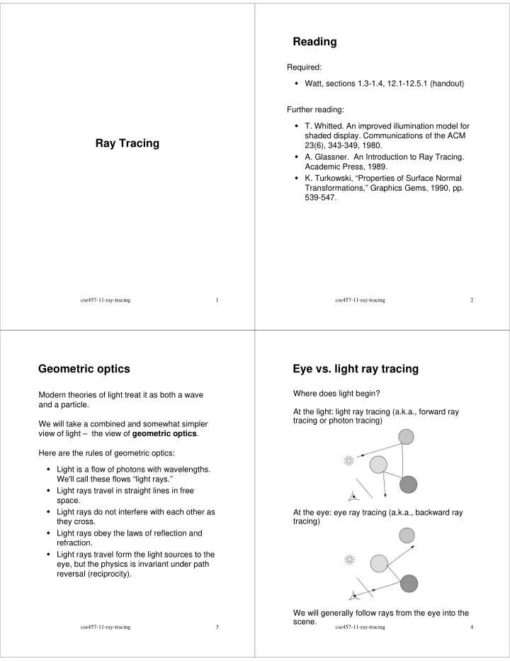
Ray Tracing

cse457-11-ray-tracing 2

Reading

Required: Watt, sections 1.3-1.4, 12.1-12.5.1 (handout) Further reading:

• T. Whitted. An improved illumination model for

shaded display. Communications of the ACM 23(6), 343-349, 1980.

• A. Glassner. An Introduction to Ray Tracing.

Academic Press, 1989.

• K. Turkowski, “Properties of Surface Normal

Transformations,” Graphics Gems, 1990, pp. 539-547.

cse457-11-ray-tracing 3

Geometric optics

Modern theories of light treat it as both a wave and a particle. We will take a combined and somewhat simpler view of light – the view of geometric optics. Here are the rules of geometric optics: Light is a flow of photons with wavelengths. We'll call these flows “light rays.” Light rays travel in straight lines in free space. Light rays do not interfere with each other as they cross. Light rays obey the laws of reflection and refraction. Light rays travel form the light sources to the eye, but the physics is invariant under path reversal (reciprocity).

cse457-11-ray-tracing 4

Eye vs. light ray tracing

Where does light begin? At the light: light ray tracing (a.k.a., forward ray tracing or photon tracing) At the eye: eye ray tracing (a.k.a., backward ray tracing) We will generally follow rays from the eye into the scene.

cse457-11-ray-tracing 5

Precursors to ray tracing

Local illumination Cast one eye ray, then shade according to light Appel (1968) Cast one eye ray + one ray to light

cse457-11-ray-tracing 6

Whitted ray-tracing algorithm

In 1980, Turner Whitted introduced ray tracing to the graphics community. Combines eye ray tracing + rays to light Recursively traces rays Algorithm:

• For each pixel, trace a primary ray in direction V to

the first visible surface.

• For each intersection, trace secondary rays:

Shadow rays in directions Li to light sources Reflected ray in direction R. Refracted ray or transmitted ray in direction T.

cse457-11-ray-tracing 7

Whitted algorithm (cont'd)

Let's look at this in stages:

Shading

A ray is defined by an origin P and a unit direction d and is parameterized by t: P + td Let I(P, d) be the intensity seen along that ray. Then: I(P, d) = Idirect + Ireflected + Itransmitted where Idirect is computed from the Phong model Ireflected = kr I (Q, R) Itransmitted = ktI (Q, T) Typically, we set kr = ks and kt = 1 – ks .

cse457-11-ray-tracing 9

Reflection and transmission

Law of reflection: θi = θr Snell's law of refraction: ηi sinθI = ηt sin θt where ηi , ηt are indices of refraction. In all cases, R and T are co-planar with d and N.

cse457-11-ray-tracing 10

Total Internal Reflection

The equation for the angle of refraction can be computed from Snell's law: What happens when ηi > ηt? When θt is exactly 90°, we say that θI has achieved the “critical angle” θc . For θI > θc , no rays are transmitted, and only reflection occurs, a phenomenon known as “total internal reflection” or TIR.

cse457-11-ray-tracing 11

Watt handout

Watt uses different symbols. Here is the translation between them: Also, Watt had some important errors that have been corrected in the handout. But, if you’re consulting the original text, be sure to refer to the errata posted on the syllabus for corrections. φ θ θ θ µ η µ η = − = = = =

i r 1 i r 2

I d

cse457-11-ray-tracing 12

Ray-tracing pseudocode

We build a ray traced image by casting rays through each of the pixels. function traceImage (scene): for each pixel (i,j) in image S = pixelToWorld(i,j) P = COP d = (S - P)/|| S – P|| I(i,j) = traceRay(scene, P, d) end for end function

Ray-tracing pseudocode, cont’d

function traceRay(scene, P, d): (t, N, mtrl) ← scene.intersect (P, d) Q ray (P, d) evaluated at t I = shade( ) R = reflectDirection( ) I ← I + mtrl.kr ∗ traceRay(scene, Q, R) if ray is entering object then ni = index_of_air nt = mtrl.index else ni = mtrl.index nt = index_of_air if (notTIR ( )) then T = refractDirection ( ) I ← I + mtrl.kt ∗ traceRay(scene, Q, T) end if return I end function

cse457-11-ray-tracing 14

Terminating recursion

Q: How do you bottom out of recursive ray tracing? Possibilities:

cse457-11-ray-tracing 15

Shading pseudocode

Next, we need to calculate the color returned by the shade function. function shade(mtrl, scene, Q, N, d): I ← mtrl.ke + mtrl. ka * scene->Ia for each light source λ do: atten = λ->distanceAttenuation( ) * λ->shadowAttenuation( ) I ← I + atten*(diffuse term + spec term) end for return I end function We are implementing the Phong shading equation:   ⋅ ⋅  

∑

s

n e a a j j d j + s j + j

atten

I = k + k L + f d L k + k ( ) ( ) ( ) N L V R

cse457-11-ray-tracing 16

Shadow attenuation

Computing a shadow can be as simple as checking to see if a ray makes it to the light source. For a point light source: function PointLight::shadowAttenuation(scene, P) d = (this.position - P).normalize() (t, N, mtrl) ← scene.intersect(P, d) Compute tlight if (t < tlight) then: atten = 0 else atten = 1 end if return atten end function

cse457-11-ray-tracing 17

Shadow attenuation (cont’d)

Q: What if there are transparent objects along a path to the light source?

Photon mapping

Combine light ray tracing (photon tracing) and eye ray tracing: …to get photon mapping.

Renderings by Henrik Wann Jensen: http://graphics.ucsd.edu/~henrik/images/caustics.html

cse457-11-ray-tracing 19

Intersecting rays with spheres

Given: The coordinates of a point along a ray passing through P in the direction d are: A unit sphere S centered at the origin defined by the equation: Find: The t at which the ray intersects S. = + = + = +

x x y y z z

x P td y P td z P td

cse457-11-ray-tracing 20

Intersecting rays with spheres

Solution by substitution: where Q: What are the solutions of the quadratic equation in t and what do they mean? Q: What is the normal to the sphere at a point (x,y,z) on the sphere?

2 2 2 2 2 2

2

1 0 ( ) ( ) ( ) 1 0

x x y y z z

x y z P td P td P td at bt c + + − = + + + + + − = + + = = + + = + + = + + −

2 2 2 2 2 2

2( ) 1

x y z x x y y z z x y z

a d d d b Pd Pd Pd c P P P

cse457-11-ray-tracing 21

Ray-plane intersection

We can write the equation of a plane as: The coefficients a, b, and c form a vector that is normal to the plane, n = [a b c]T. Thus, we can re- write the plane equation as: We can solve for the intersection parameter (and thus the point):

= + + + D cz by ax

cse457-11-ray-tracing 22

Ray-triangle intersection

To intersect with a triangle, we first solve for the equation of its supporting plane. How might we compute the (un-normalized) normal? Given this normal, how would we compute D? Using these coefficients, we can solve for Q. Now, we need to decide if Q is inside or outside of the triangle.

cse457-11-ray-tracing 23

3D inside-outside test

One way to do this “inside-outside test,” is to see if Q lies on the left side of each edge as we move counterclockwise around the triangle. How might we use cross products to do this?

cse457-11-ray-tracing 24

2D inside-outside test

Without loss of generality, we can perform this same test after projecting down a dimension: If Q’ is inside of A’B’C’, then Q is inside of ABC. Why is this projection desirable? Which axis should you “project away”?

cse457-11-ray-tracing 25

Barycentric coordinates

As we’ll see in a moment, it is often useful to represent Q as an affine combination of A, B, and C: where: We call α, β, and γ, the barycentric coordinates

• f Q with respect to A, B, and C.

Q A B C α β γ = + + 1 α β γ + + =

cse457-11-ray-tracing 26

Barycentric coordinates

Given a point Q that is inside of triangle ABC, we can solve for Q’s barycentric coordinates in a simple way: How can cross products help here? In the end, these calculations can be performed in the 2D projection as well! α β γ = = = Area( ) Area( ) Area( ) Area( ) Area( ) Area( ) QB C AQC AB Q AB C AB C AB C

cse457-11-ray-tracing 27

Interpolating vertex properties

The barycentric coordinates can also be used to interpolate vertex properties such as: material properties texture coordinates normals For example: Interpolating normals, known as Phong interpolation, gives triangle meshes a smooth shading appearance. (Note: don’t forget to normalize interpolated normals.)

α β γ = + + ( ) ( ) ( ) ( )

d d d d

k Q k A k B k C

cse457-11-ray-tracing 28

Epsilons

Due to finite precision arithmetic, we do not always get the exact intersection at a surface. Q: What kinds of problems might this cause? Q: How might we resolve this?

cse457-11-ray-tracing 29

Summary

What to take home from this lecture:

• The meanings of all the boldfaced terms.
• Enough to implement basic recursive ray

tracing.

• How reflection and transmission directions

are computed.

• How ray--object intersection tests are

performed on spheres, planes, and triangles

• How barycentric coordinates within triangles

are computed

• How ray epsilons are used.