Reading Reading: Angel 5.6, 9.10.3 Optional reading: Foley, van - PDF document

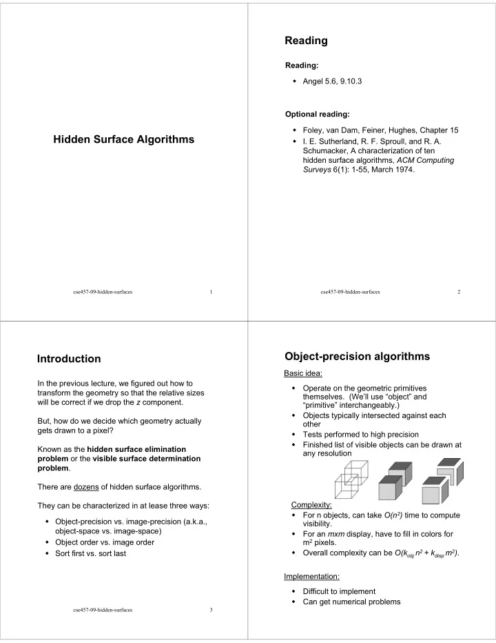
Reading Reading: � Angel 5.6, 9.10.3 Optional reading: � Foley, van Dam, Feiner, Hughes, Chapter 15 Hidden Surface Algorithms � I. E. Sutherland, R. F. Sproull, and R. A. Schumacker, A characterization of ten hidden surface algorithms, ACM Computing Surveys 6(1): 1-55, March 1974. cse457-09-hidden-surfaces 1 cse457-09-hidden-surfaces 2 Object-precision algorithms Introduction Basic idea: In the previous lecture, we figured out how to Operate on the geometric primitives transform the geometry so that the relative sizes � themselves. (We’ll use “object” and will be correct if we drop the z component. “primitive” interchangeably.) Objects typically intersected against each � But, how do we decide which geometry actually other gets drawn to a pixel? Tests performed to high precision � Finished list of visible objects can be drawn at Known as the hidden surface elimination � any resolution problem or the visible surface determination problem . There are dozens of hidden surface algorithms. Complexity: They can be characterized in at lease three ways: For n objects, can take O(n 2 ) time to compute � � Object-precision vs. image-precision (a.k.a., visibility. object-space vs. image-space) For an mxm display, have to fill in colors for � � Object order vs. image order m 2 pixels. Overall complexity can be O(k obj n 2 + k disp m 2 ) . � Sort first vs. sort last � Implementation: Difficult to implement � Can get numerical problems � cse457-09-hidden-surfaces 3

Image-precision algorithm Object order vs. image order Basic idea: Object order: � Find the closest point as seen through each � Consider each object only once, draw its pixel pixels, and move on to the next object. � Calculations performed at display resolution � Might draw to the same pixel multiple times. � Does not require high precision Complexity: Image order: � Naïve approach checks all n objects at every � Consider each pixel only once, find nearest pixel. Then, O(n m 2 ). object, and move on to the next pixel. � Better approaches check only the objects � Might compute relationships between objects that could be visible at each pixel. Let’s say, multiple times. on average, d objects project to each pixel (a.k.a., depth complexity). Then, O(d m 2 ) . Implementation: � Very simple to implement. • Used a lot in practice. cse457-09-hidden-surfaces 5 cse457-09-hidden-surfaces 6 Sort first vs. sort last Three hidden surface algorithms Sort first: � Z-buffer � Ray casting � Find some depth-based ordering of the objects relative to the camera, then draw � Binary space partitioning (BSP) trees back to front. � Build an ordered data structure to avoid duplicating work. Sort last: � Determine depth observed at each pixel and draw the color corresponding to the closest depth � Can be done by considering all depths together or by “lazily” keeping track of depths as they arrive. cse457-09-hidden-surfaces 7 cse457-09-hidden-surfaces 8

Z-buffer Rasterization The Z-buffer or depth buffer algorithm [Catmull, 1974] The process of filling in the pixels inside of a is probably the simplest and most widely used. polygon is called rasterization . Here is pseudocode for the Z-buffer hidden surface During rasterization, the z value and shade s can algorithm: be computed incrementally (fast!). for each pixel (i,j) do Z-buffer [i,j] ← FAR Framebuffer[i,j] ← <background color> end for for each polygon A do for each pixel in A do Compute depth z and shade s of A at (i,j) if z > Z-buffer [i,j] then Z-buffer [i,j] ← z Curious fact: Framebuffer[i,j] ← s end if Described as the “brute-force image space � end for algorithm” by [SSS] end for Mentioned only in Appendix B of [SSS] as a � point of comparison for huge memories, but written off as totally impractical. Q : What should FAR be set to? Today, Z-buffers are commonly implemented in hardware. cse457-09-hidden-surfaces 9 cse457-09-hidden-surfaces 10 Z-buffer: Analysis Ray casting Classification? � Easy to implement? � Easy to implement in hardware? � Incremental drawing calculations (uses coherence)? � Pre-processing required? � On-line (doesn’t need all objects before drawing � begins)? If objects move, does it take more work than normal � to draw the frame? If the viewer moves, does it take more work than � normal to draw the frame? Typically polygon-based? Idea: For each pixel center P ij � Efficient shading (doesn’t compute colors of hidden � surfaces)? � Send ray from eye point (COP), C , through P ij into scene. Handles transparency? � Handles refraction? � Intersect ray with each object. � � Select nearest intersection. cse457-09-hidden-surfaces 11 cse457-09-hidden-surfaces 12

Ray casting, cont. Ray casting: Analysis � Classification? � Easy to implement? � Easy to implement in hardware? � Incremental drawing calculations (uses coherence)? � Pre-processing required? � On-line (doesn’t need all objects before drawing begins)? Implementation: � If objects move, does it take more work than normal to draw the frame? � Might parameterize each ray: � If the viewer moves, does it take more work than r (t) = C + t ( P ij - C ) normal to draw the frame? � Typically polygon-based? � Each object O k returns t k > 0 such that first � Efficient shading (doesn’t compute colors of intersection with O k occurs at r ( t k ). hidden surfaces)? � Handles transparency? Q : Given the set { t k } what is the first intersection � Handles refraction? point? Note: these calculations generally happen in world coordinates. No projective matrices are applied. cse457-09-hidden-surfaces 14 Binary-space partitioning (BSP) BSP tree creation trees C A B D Idea: � Do extra preprocessing to allow quick display from any viewpoint. Key observation: A polygon A is painted in correct order if � Polygons on far side of A are painted first � A is painted next � Polygons in front of A are painted last. cse457-09-hidden-surfaces 15 cse457-09-hidden-surfaces 16

BSP tree creation (cont’d) BSP tree display procedure MakeBSPTree : procedure DisplayBSPTree: takes PolygonList L Takes BSPTree T returns BSPTree if T is empty then return Choose polygon A from L to serve as root Split all polygons in L according to A if viewer is in front (on pos. side) of T.node node ← A DisplayBSPTree(T. _____ ) node.neg ← MakeBSPTree (Polygons on neg. side of A) Draw T.node node.pos ← MakeBSPTree (Polygons on pos. side of A) return node DisplayBSPTree(T._____) end procedure else DisplayBSPTree(T. _____) Draw T.node DisplayBSPTree(T. _____) Note: Performance is improved when fewer end if polygons are split --- in practice, best of ~ 5 end procedure random splitting polygons are chosen. Note: BSP is created in world coordinates. No projective matrices are applied before building tree. cse457-09-hidden-surfaces 18 BSP trees: Analysis Cost of Z-buffering Z-buffering is the algorithm of choice for hardware Classification? � rendering, so let’s think about how to make it run as Easy to implement? � fast as possible… Easy to implement in hardware? � Incremental drawing calculations (uses coherence)? � The steps involved in the Z-buffer algorithm are: Pre-processing required? � On-line (doesn’t need all objects before drawing • Send a triangle to the graphics hardware. � begins)? • Transform the vertices of the triangle using the If objects move, does it take more work than normal modeling matrix. � to draw the frame? • Shade the vertices. If the viewer moves, does it take more work than � • Transform the vertices using the projection normal to draw the frame? matrix. Typically polygon-based? � • Set up for incremental rasterization Efficient shading (doesn’t compute colors of hidden calculations � surfaces)? • Rasterize and update the framebuffer Handles transparency? � according to z . Handles refraction? � What is the overall cost of Z-buffering? cse457-09-hidden-surfaces 19 cse457-09-hidden-surfaces 20

Cost of Z-buffering, cont’d Visibility tricks for Z-buffers We can approximate the cost of this method as: Given this cost function: k bus v bus + k xform v xform + k shade v shade + k setup ∆ rast + d m 2 k bus v bus + k xform v xform + k shade v shade + k setup ∆ rast + d m 2 what can we do to accelerate Z-buffering? Accel method v bus v xform v shade ∆ rast d m Where: k bus = bus cost to send a vertex v bus = number of vertices sent over the bus k xform = cost of transforming a vertex v xform = number of vertices transformed k shade = cost of shading a vertex v shade = number of vertices shaded k setup = cost of setting up for rasterization ∆ rast = number of triangles being rasterized d = depth complexity (average times a pixel is covered) m 2 = number of pixels in frame buffer cse457-09-hidden-surfaces 21 cse457-09-hidden-surfaces 22 Summary What to take home from this lecture: � Classification of hidden surface algorithms � Understanding of Z-buffer, ray casting, and BSP tree hidden surface algorithms � Familiarity with some Z-buffer acceleration strategies cse457-09-hidden-surfaces 23