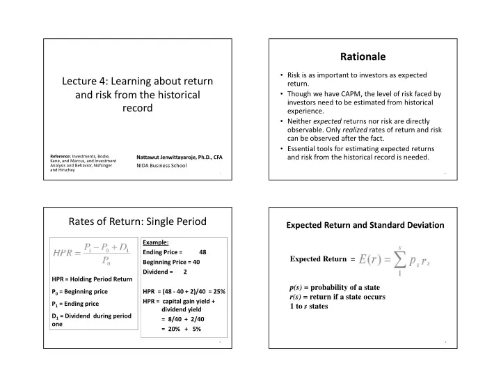
Rationale Risk is as important to investors as expected Lecture 4: - PowerPoint PPT Presentation

Rationale • Risk is as important to investors as expected Lecture 4: Learning about return return. and risk from the historical • Though we have CAPM, the level of risk faced by investors need to be estimated from historical record experience. • Neither expected returns nor risk are directly observable. Only realized rates of return and risk can be observed after the fact. • Essential tools for estimating expected returns and risk from the historical record is needed. Reference : Investments, Bodie, Nattawut Jenwittayaroje, Ph.D., CFA Kane, and Marcus, and Investment Analysis and Behavior, Nofsinger NIDA Business School and Hirschey 1 2 Rates of Return: Single Period Expected Return and Standard Deviation Example: Ending Price = 48 Expected Return = Beginning Price = 40 Dividend = 2 HPR = Holding Period Return p(s) = probability of a state P 0 = Beginning price HPR = (48 - 40 + 2)/40 = 25% r(s) = return if a state occurs HPR = capital gain yield + P 1 = Ending price 1 to s states dividend yield D 1 = Dividend during period = 8/40 + 2/40 one = 20% + 5% 3 4

Variance or Dispersion of Returns Expected Returns: Example State Prob. of State r in State 1 .1 -.05 (or 5%) 2 .2 .05 3 .4 .15 Standard deviation = [variance] 1/2 4 .2 .25 Using Our Example : 5 .1 .35 Var =[(.1)(-.05-.15) 2 +(.2)(.05- .15) 2 ...+ .1(.35-.15) 2 ] E( r ) = (.1)(-.05) + (.2)(.05)...+ (.1)(.35) Var= .01199 E( r ) = .15 = 15% S.D.= [ .01199] 1/2 = .1095 = 10.95% 5 6 Mean and Variance of Historical Returns Mean and Variance of Historical Returns • In forward-looking analysis so far, we determine a set of relevant scenarios and associated investment outcomes (i.e., rates of return) and probability. Expected return is arithmetic average • In contrast, asset and portfolio return histories or arithmetic average of rates of return come in the form of time series of past realized returns that do not explicitly provide the probabilities of those observed returns; we observe only dates and associated holding period returns. • Therefore, when we use historical data, we treat each observation as an equally likely scenario. 7 8

The Normal Distribution The Normal Distribution • Investment management is far more tractable when asset rates of return can be well approximated by the normal distribution. • First, it’s symmetric. Therefore, measuring risk as the SD of returns is adequate . • Second, when assets with normally distributed returns are mixed, the resulting portfolio return is also normally distributed. • Third, only two parameters (mean and SD) have to be estimated to obtain the probabilities of future scenarios. A graph of the normal curve with mean of 10% and the • How closely actual return distributions fit the normal standard deviation of 20%. curve……. 9 10 Normal and Skewed Distribution (mean = 6% SD = 17%) Normal and Fat Tails Distributions (mean = .1 SD =.2) Skewness measures the Kurtosis is a measure of degree of asymmetry the degree of “fat tails”. Positive (negative) skewness  SD overestimates (underestimate) risk. 11 12

Histograms of Rates of Return History of Rates of Returns of Asset Classes for Generations, 1926- 2005 for 1926-2005 • The asset classes with higher volatility (i.e., SD) provided higher average returns  investors demand a risk premium to bear risk. 13 14 History of Excess Returns of Asset Classes for Generations, Excess Returns and Risk Premiums 1926- 2005 • How much should you invest in a risky asset (e.g., stocks)….. • How much of an expected reward is offered for the risk involved in investing money in a stock…. • We measure the reward as the difference between the expected holding-period return on the stock and the risk-free rate  “ risk premium ”. • The difference in any particular period between the actual rate of return on a risky asset and the risk- free rate  “excess return” . 15 16

History of Excess Returns of Asset Classes for Generations, 1926- 2005 • The average excess return was positive for every sub- periods. Average excess returns of large stocks in the last 40 years suggest a risk premium of 6%-8% • The skews of the two large stock portfolios are significantly negative, -0.62 and -0.70. • Negative skews imply SD underestimates the actual level of risk. • Fat tails are observed for five assets during 1926-2005. • The serial correlation is practically zero for four of the five portfolios, supporting market efficiency. 17