SLIDE 1 Random band matrices
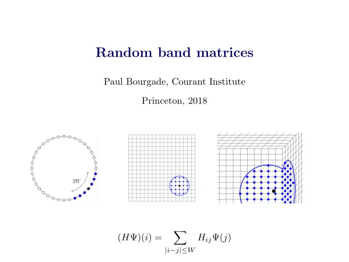
Paul Bourgade, Courant Institute Princeton, 2018 (HΨ)(i) =
HijΨ(j)
SLIDE 2 Integrable models : diagonal matrices (W = 0) or the Gaussian Orthogonal Ensemble (W = N/2, Gaussian entries), which satisfies : (i) Semicircle law as N → ∞ (Wigner) : ρ(E) = 1 2π
(ii) Eigenvalues locally converge (Gaudin, Mehta, Dyson) :
δNρ(E)(λk−E) → Sine1. (iii) Eigenvectors are uniform on the sphere, essentially supported on all sites (delocalization). The L´ evy-Borel law holds : for any q2 = 1, √ Nuk, q − →
N→∞ N (0, 1).
SLIDE 3
For d = 1, 2, 3, vertices are elements of Λ = 1, Nd and H = (Hij)i,j∈Λ are centered, real, independent up to the symmetry Hij = Hji. Band width W : Hij = 0 if |i − j| > W. Localization (eigenvector support length ℓ ≪ N) ? Conjecture : transition at some critical band width Wc(N). Localization for W ≪ Wc, delocalization for W ≫ Wc, where Wc = N 1/2 for d = 1 (ℓ ∼ min(W 2, N)), (log N)1/2 for d = 2 (ℓ ∼ min(eW 2, N)), O(1) for d = 3. Simultaneous transition of eigenvalues statistics, from Poisson to GOE.
SLIDE 4
Context
SLIDE 5 Context Mean field models Band matrices Probabilistic QUE
A spacially confined quantum mechanical system can only take certain discrete values of energy. Uranium-238 : These values are eigenvalues of a certain self-adjoint operator. Wigner’s universality idea. The local spectral sta- tistics of highly correlated quantum systems are given by the random matrix statistics of the same symmetry
- type. Random matrix statistics are ”universal” probabi-
lity laws. Wigner’s vision is not proved for any realistic Hamiltonian. At least one model beyond mean-field ?
SLIDE 6 Context Mean field models Band matrices Probabilistic QUE
Problem 1 : GOE and delocalization with no randomness. Bohigas-Giannoni-Schmit conjecture : if the billard is chaotic, GOE-type repulsion of eigenvalues. Helmholtz equation : −∆ψn = λnψn. Weyl law : |{i : λi ≤ λ}| ∼
λ→∞ area(D) 4π
λ. Spacings statistics : χ(n) = 1 n
δ
4π area(D) (λi+1−λi).
(Numerics : A. Backer) Delocalization on average (quantum ergodicity) is proved. GOE is not.
SLIDE 7 Context Mean field models Band matrices Probabilistic QUE
Problem 2 : GOE and delocalization with non-trivial geometry. Anderson’s model for metal-insulator transition : H = −∆ + λVω
- n Zd ∩ [−L, L]d, random i.i.d. potential.
Depending on λ and d, two distinct regimes : (i) Localization for large λ, any d, by multiscale analysis (Frohlich-Spencer), fractional moment (Aizenman-Molchanov). Poisson statistics (Minami). (ii) Delocalization and GOE (e.g., small λ for d = 3) ? For Anderson, localization was the new phenomenon. Mathematically speaking, delocalization is harder : for all dimensions, nothing is proved. Minami showed that Exponential decay of the resolvent implies Poisson statistics. Mechanism for GOE statistics in the delocalized phase ?
SLIDE 8 Context Mean field models Band matrices Probabilistic QUE
Delocalization, GOE, for at least one model beyond mean-field ? Content :
- 1. Mean-field models.
- 2. Results for band matrices.
- 3. Elements of proof for the delocalized regime, d = 1, W ≫ N 3/4.
Heuristics for transition exponents.
SLIDE 9
Mean field models
SLIDE 10 Context Mean field models Band matrices Probabilistic QUE
Wigner matrices : eigenvalues universality. N × N symmetric, E(Hij) = 0, E(H2
ij) = 1
N , higher moments are finite but arbitrary.
Theorem (2014)
For any E ∈ (−2, 2),
i δNρ(E)(λk−E) → Sine1. Johansson (2000) : Hermitian case with large Gaussian component, HCIZ formula Erd˝
ech´ e-Ramirez-Schlein-Yau (2009), Hermitian case, reverse heat flow Tao-Vu (2009) : Hermitian case, moment matching Erd˝
- s-Schlein-Yau (2009) : general case with averaging over E, relative entropy method
B.-Erd˝
- s-Yau-Yin (2014) : general case, fixed energy, coupling method
Erd˝
- s-Schlein-Yau dynamic idea, use Dyson Brownian Motion :
dHt = dBt √ N − 1 2Htdt, H0 Wigner.
SLIDE 11 Context Mean field models Band matrices Probabilistic QUE
Step 1 : relaxation. For t ≫ N −1+ε, local equilibrium is reached. Relies on coupled dynamics. Let x(0) be the spectrum of H0, y(0) of GOE. dxi/dyi =
N dBi(t) + 1 N
1 xi/yi − xj/yj dt. Then δℓ(t) = xℓ(t) − yℓ(t) satisfies the parabolic equation ∂tδℓ(t) =
δk(t) − δℓ(t) N(xk(t) − xℓ(t))(yk(t) − yℓ(t)). H¨
- lder regularity = universality. This coupling argument is local, it gives
relaxation for any initial condition (Landon-Sosoe-Yau, Erd˝
Step 2 : density. For t ≪ N − 1
2 −ε, the local eigenvalues distribution has
almost not changed. Relies on the matrix structure (Itˆ
step fails for non mean field models.
SLIDE 12 Context Mean field models Band matrices Probabilistic QUE
Wigner matrices : eigenvectors universality. Let u1, . . . , uN be the eigenvectors associated to λ1 ≤ · · · ≤ λN. By the density step, universality of bulk eigenvectors in the perturbative setting E(( √ NHij)3) = 0, E(( √ NHij)4) = 3 )(Knowles-Yin, Tao-Vu, 2011).
Theorem (B-Yau, 2013)
For any deterministic k, q ∈ RN , √ Nq, uk converges to a Gaussian. Relaxation step for eigenvectors ? Joint eigenvalues/eigenvectors dynamics
(Bru, 1989)
dλk = dBkk √ N + 1 N
1 λk − λℓ dt duk = 1 √ N
dBkℓ λk − λℓ uℓ − 1 2N
dt (λk − λℓ)2 uk
SLIDE 13 Context Mean field models Band matrices Probabilistic QUE
Random walk in a dynamic random environment. Configuration η of n points on 1, N. Usual notations :
- ηk, number of points at k
- ηij configuration obtained by moving a point from i to j.
Define zk(t) = √ Nq, uk(t) and f(η) = ft,λ(η) = E N
z2ηk
k
| λ0→∞
N
N 2ηk
k
Lemma
∂tf(η) =
2ηi(1+2ηj) f(ηij) − f(η) N(λi(t) − λj(t))2 . H¨
- lder regularity for t ≫ N −1+ε means moments are Gaussian.
SLIDE 14 Context Mean field models Band matrices Probabilistic QUE
Numerics : L. Benigni
SLIDE 15 Context Mean field models Band matrices Probabilistic QUE
The dynamic approach applies beyond Wigner matrices. Examples : (i) Matrices with general mean, variance profile, summable decay of correlations (Ajanki-Erd˝
uger-Schr¨
(ii) Sparse random graphs of Erd˝
- s-Renyi-type (Erd˝
- s-Knowles-Yau-Yin,
Lee-Schnelli, Huang-Landon-Yau) and d-regular models (Bauerschmidt-Huang-Knowles-Yau, B-Huang-Yau)
(iii) Convolution, free probability model D1 + U ∗D2U, U uniform on O(N) (Bao-Erd˝
The above matrix models are all mean-field.
SLIDE 16
Random band matrices
SLIDE 17 Context Mean field models Band matrices Probabilistic QUE
We say that an eigenvector ψ is subexponentially localized at scale ℓ if there exists ε > 0, I ⊂ 1, N, |I| ≤ ℓ, such that
α∈I |ψ(α)|2 < e−N ε.
Conjecture : Wc = N 1/2 for d = 1 for bulk eigenvectors
- 1. Based on numerics (Casati-Molinari-Izrailev, 1990)
- 2. Theoretical evidence from supersymmetric method (Fyodorov-Mirlin, 1991)
Corresponding localization length : ℓ ≈ W 2. Analogy with the Anderson model H = −∆ + λVω : λ ≈ W −1. Consistent with localization length λ−2 for d = 1, eλ−2 for d = 2.
SLIDE 18 Context Mean field models Band matrices Probabilistic QUE
Results on microscopic scale.
- 1. Edge behavior
- 2. Gaussian models with specific variance profile
- 3. Localization for general models
- 4. Delocalization for general models
- 1. Edge behavior. The transition at W ≈ N 5/6 was made rigorous by a
subtle method of moments.
Theorem (Sodin, 2010)
If W ≫ N
5 6 , then N 2/3(λN − 2) converges to the Tracy-Widom
5 6 , this does not hold.
SLIDE 19 Context Mean field models Band matrices Probabilistic QUE
- 2. Gaussian models with specific variance profile, supersymmetry.
Covariance structure E(HijHℓk) = 1i=k,j=ℓJij where Jij = (−W 2∆ + 1)−1
ij .
Essentially a 1d band matrix of width W. Define F2(E1, E2) = E (det(E1 − H) det(E2 − H)) .
Theorem (Shcherbina-Shcherbina, 2014-2017)
(D2)−1F2
x Nρ(E), E − x Nρ(E)
if N ε < W < N
1 2 −ε
sin(2πx) 2πx
if N
1 2 +ε < W < N
Proof idea : representation for the left hand side (N = 2n + 1)
2
n
−n+1 Tr(Xj−Xj−1)2− 1 2
n
−n Tr(Xj+ iΛE 2
+i
Λx Nρ(E )2
n
det(Xj−i∆E 2 )dXj, where ∆E = diag(E, E), ∆x = diag(x, −x). Then steepest descent. Other results, 3d density of states (Disertori-Pinson-Spencer), 1d pair correlation for W of order N (Shcherbina).
SLIDE 20 Context Mean field models Band matrices Probabilistic QUE
- 3. Localization for general models. The following implies localization
for W ≪ N 1/8.
Theorem (Schenker (2009))
Let µ > 8. There exists τ > 0 such that for large enough N, for any α, β ∈ 1, N one has E
1≤k≤N
|uk(α)uk(β)|
W µ .
This was improved to W ≪ N 1/7 for some specific Gaussian model
(Peled-Schenker-Shamis-Sodin).
The Poisson eigenvalues statistics are still unknown.
SLIDE 21 Context Mean field models Band matrices Probabilistic QUE
- 4. Delocalization for general models. An advanced analysis of the
resolvent of band matrices gives an average form of delocalization : For W ≫ N 7/9 and ℓ ≪ N, the fraction of eigenvectors localized on scale ℓ vanishes as N → ∞ (Erd˝
- s-Knowles-Yau-Yin 2012, He-Marcozzi 2018).
Theorem (B-Yau-Yin, 2018)
Assume W ≫ N 3/4. (a) Universality. For any E ∈ (−2, 2),
i δNρ(E)(λk−E) → Sine1.
(b) Delocalization. For any unit bulk eigenvector ψ, ψ∞ < N − 1
2 +ε.
(c) Quantum unique ergodicity. There exists c > 0 such that for any interval I ⊂ 1, N, |I| > W,
N )
N .
Previously proved for W ≥ cN in (B-Erd˝
- s-Yau-Yin 2016), where a mean-field
reduction method was introduced.
SLIDE 22 Context Mean field models Band matrices Probabilistic QUE
Quantum unique ergodicity (QUE) is the main mechanism for GOE. QUE conjecture (Rudnick, Sarnak). If M is compact and negatively curved, and (ψk)k≥1 the Laplacian eigenfunctions,
|ψk(x)|2µ(dx) − →
k→∞
µ(dx). Known : arithmetic QUE (Lindenstrauss), more general cases in an average sense, quantum ergodicity (Shnirelman, Zelditch, Colin de Verdi`
ere), quantum
ergodicity for random regular graphs (Anantharaman-Le Masson). (i) QUE implies GOE (ii) Heuristics : QUE and GFF give the threshold Wc. (iii) Averaged QUE and DBM imply QUE
SLIDE 23
Probabilistic QUE
SLIDE 24 Context Mean field models Band matrices Probabilistic QUE
From QUE to GOE : mean-field reduction. Let He =
B∗ B D
W × W, and ψj the eigenvector associated with λj : Hψj = λjψj. Denote ψj =
pj
Qλjwj = λjwj where Qe = A − B∗(D − e)−1B. Let ξe
k’s be the eigenvalues of Qe
dξe
k
de = − pk2
2
wk2
2
. Knowing QUE, GOE for band follows from GOE for Qe by parallel projection. Representation of eigenvalues of Qe as a function of e :
SLIDE 25 Context Mean field models Band matrices Probabilistic QUE
QUE and GFF : heuristics. QUE for an eigenvector ψ of H is obtained from QUE for Qe and a simple patching : (1) If QUE holds for all Qe, π[1,W/2]ψ2 ≈ π[W/2,W ]ψ2. (2) Patching this equality over N
W pairs of intervals gives a flat ψ.
(3) Central limit for sum of errors :
W · 1 √ W ≪ 1 when W ≫ N 1/2.
For any dimension, decompose 1, Nd into N
W
d cubes Cv of side W. Let Xv =
|ψ(i)|2. Good model for (Xv)v : independent N (0, W d
N 2d ) increments over adjacent
cubes, conditioned to (Xvi+1 − Xvi) = 0 for any closed path. This model is simply the Gaussian free field on 1, N/Wd, with density e− N2d
2W d
QUE holds when Var(Xv)1/2 ≪ E(Xv). For the GFF model, this means W ≫ (log N)1/2 (d = 2), W ≫ 1 (d = 3).
SLIDE 26 Context Mean field models Band matrices Probabilistic QUE
From averaged QUE to QUE : dynamics. Consider the Dyson Brownian Motion : dQ(t) = dBt
√n . Assume Q = Q0 satisfies an averaged
QUE in the sense that
|I|
((Q − z)−1)ii − 1 nTr(Q − z)−1
Lemma
Quantum unique ergodicity holds for t ≫ n−β : if ψt is any eigenvector of Q(t), with overwhelming probability
(ψt(α)2 − 1 n)
The initial averaged QUE estimate is hard to obtain for A − B∗(D − e)−1B (singularity). Analysis of a generalized Green’s function (B-Yang-Yau-Yin,
Yang-Yin).
SLIDE 27 Context Mean field models Band matrices Probabilistic QUE
pij =
ui(α)uj(α) (i = j), pii =
ui(α)2 − |I| n , For any given configuration η, double the set of particles and consider the set of perfect matchings Gη, each graph G with edges E(G). Define
1 M(η) E
G∈Gη
P(G) | λ , M(η) =
n
(2ηi)!!,
Lemma
∂t f(η) =
2ηi(1 + 2ηj)
f(η) N(λi(t) − λj(t))2 .
SLIDE 28
Beyond mean field, one model with proved GOE and delocalization : random band matrices for W ≫ N 3/4 (d = 1) and W ≫ N 1−κ for d = 2, 3. The exponents are not optimal. Quantum unique ergodicity gives GOE (localization gives Poisson statistics). For the proof of quantum unique ergodicity, new integrable dynamics connect to random walks in time-dependent random environments. One major question is random matrix statistics in a deterministic setting.