R u t c o r R esearch R e p o r t Logical Analysis of Data: - - PDF document

R u t c o r Research R e p o r t

RUTCOR Rutgers Center for Operations Research Rutgers University 640 Bartholomew Road Piscataway, New Jersey 08854-8003 Telephone: 732-445-3804 Telefax: 732-445-5472 Email: rrr@rutcor.rutgers.edu http://rutcor.rutgers.edu/∼rrr

Logical Analysis of Data: Classification with Justification

Endre BOROSa Yves CRAMAb Peter L. HAMMERc Toshihide IBARAKId Alexander KOGANe Kazuhisa MAKINOf

RRR 5-2009, February 2009

aRUTCOR, Rutgers Center for Operations Research, Piscataway, NJ

08854-8003, USA, boros@rutcor.rutgers.edu

bHEC Management School, University of Li`

ege, Boulevard du Rectorat 7 (B31), B-4000 Li` ege, Belgium, Yves.Crama@ulg.ac.be

cOur colleague and friend, Peter L. Hammer passed away in a tragic car

accident in 2006, while we were working on this manuscript.

dDepartment

• f

Informatics, School

• f

Science and Technology, Kwansei Gakuin University, 2-1 Gakuen, Sanda, Japan 669-1337, ibaraki@kwansei.ac.jp

eDepartment of Accounting, Business Ethics and Information Systems,

Rutgers Business School, Rutgers University, Newark, NJ 07102, and RUT- COR, Rutgers Center for Operations Research, Piscataway, NJ 08854-8003, USA, kogan@rutgers.edu

fGraduate School of Information Science and Technology, University of

Tokyo, Tokyo, 113-8656, Japan, makino@mist.i.u-tokyo.ac.jp

Rutcor Research Report

RRR 5-2009, February 2009

Logical Analysis of Data: Classification with Justification

Endre BOROS Yves CRAMA Peter L. HAMMER Toshihide IBARAKI Alexander KOGAN Kazuhisa MAKINO

• Abstract. Learning from examples is a frequently arising challenge, with a large

number of algorithms proposed in the classification and data mining literature. The evaluation of the quality of such algorithms is usually carried out ex post, on an experimental basis: their performance is measured either by cross validation on benchmark data sets, or by clinical trials. None of these approaches evaluates di- rectly the learning process ex ante, on its own merits. In this paper, we discuss a property of rule-based classifiers which we call “justifiability”, and which focuses on the type of information extracted from the given training set in order to classify new

• bservations. We investigate some interesting mathematical properties of justifiable
• classifiers. In particular, we establish the existence of justifiable classifiers, and we

show that several well-known learning approaches, such as decision trees or nearest neighbor based methods, automatically provide justifiable classifiers. We also iden- tify maximal subsets of observations which must be classified in the same way by every justifiable classifiers. Finally, we illustrate by a numerical example that using classifiers based on “most justifiable” rules does not seem to lead to overfitting, even though it involves an element of optimization. Acknowledgements: The authors are thanking the sponsors of the DIMACS-RUTCOR Workshop on Boolean and Pseudo-Boolean Functions in Memory of Peter L. Hammer (Jan- uary 19-22, 2009, Rutgers University) for the opportunity to get together and finalize this long overdue manuscript.

Page 2 RRR 5-2009

1 Introduction

An increasing number of machine learning tools assist daily decisions – including fully or partly automated systems used by banks (e.g., evaluation of loan worthiness, detection of credit card fraud), by communications companies (detection of illegal cellular phone use), by law enforcement authorities (criminal or terrorist profiling), or in medicine (pre-screening

• f patients). Most of these situations are governed by the conditions and rules of highly

complex environments where, unlike in physics or chemistry, fundamental laws are rarely available to help the decision-maker in the process of reaching his conclusions. Instead, most

• f systems derive their intelligence from databases of historical cases, described in terms of

their most salient attributes. Sophisticated data analysis techniques and learning algorithms are used to derive diagnosis rules, or profile descriptions which are then implemented in practice. The more these systems affect our everyday life, the more controversies and conflicts may arise: in certain cases, the consequences of potential mistakes may indeed be very expen- sive, or drastic in some other way (think for instance of a serious disease being diagnosed belatedly, due to a faulty screening decision). In such cases, the organization applying such automated tools might be forced to justify itself, and to demonstrate that it had solid, ob- jective arguments to formulate its diagnosis. But in fact, it is usually not entirely clear what could amount to an acceptable justification of a classification rule, and how a classifier could be certified to provide justifiable classifications for each of its future applications. In this paper, we want to argue that some minimal requirements for “justifiability” are satisfied by the classification rules introduced by Crama, Hammer and Ibaraki [13], and subsequently developed into a rich classification framework under the name of Logical Analysis of Data, or LAD (see for instance [5, 7, 8, 9, 10, 11, 19], etc.). We also aim at collecting some fundamental properties of LAD-type classification rules which have not appeared elsewhere, yet. Finally, we want to clarify the relation between these rules and certain popular classification rules used in the machine learning literature, such as the rules computed by nearest neighbor classification algorithms or decision trees. The paper is organized as follows. In Section 2, we rely on a small example to explain in some detail, but informally, what we mean by a “justifiable” classification rule. Section 3 recalls useful facts about partially defined Boolean functions and their extensions, and in- troduces the main concepts and definitions used in LAD. In particular, it introduces an interesting family of Boolean classifiers called bi-theories, which can be built on elementary rules called patterns and co-patterns. Our main results are presented in Section 4, together with relevant examples and interpretations, but without the proofs which are collected to- gether in Appendix A, so as to facilitate the reading. In these sections, we establish some

• f the main structural properties of patterns, co-patterns and bi-theories, and we examine

their computational complexity. We also show that decision trees and nearest neighbor pro- cedures fall under this generic LAD setting. In spite of their simplicity, we provide empirical evidence in Section 5 that the LAD rules perform and generalize well in a variety of applied

• situations. Section 6 mentions a number of challenging open questions.

RRR 5-2009 Page 3

2 An example

Let us first illustrate the basic issues and ideas on a small example. (Although this example is very small and artificial, we note that similar issues arise in many real situations where a simple scoring method is used to derive classifications.) We assume that seven suspected cases of a rare disease have been documented in the medical literature. Three of the cases (patients A, B, and C) were “positive cases” who eventually developed the disease; the other four suspicious cases (patients T, U, V and W) turned out to be “negative”, healthy cases. The following table displays the available data; each case is described by binary values indicating the presence or absence of four different symptoms. Symptoms Patients x1 x2 x3 x4 A 1 1 1 B 1 1 1 C 1 1 1 T 1 1 U 1 1 V 1 1 W 1 1 Both Dr Perfect (or Dr P in short) and Dr Rush (or Dr R in short) have access to this table, and both develop their own diagnosis rules by analyzing the data set. Dr R notices that the positive cases, and only those, exhibit 3 out of the 4 symptoms; so, he derives this as a diagnosis rule, i.e., he decides to consider a patient described by the symptom vector x = (x1, x2, x3, x4) as a “positive case” if x1 + x2 + x3 + x4 ≥ 3. Dr P performs a different analysis: he regards symptom x3 as irrelevant, and he values symptom x2 as twice more important than the other ones. Consequently, he diagnoses a patient as “positive” if x1 + 2x2 + x4 ≥ 3. It is easy to check that both doctors have derived a “perfect” diagnosis rule in the sense that all cases in the small data base are correctly diagnosed by these rules. Hence, both doctors could feel that their classification rules are well-grounded, given the current state of knowledge. Still, the above two diagnosis rules are not identical, and therefore they may certainly provide contradictory conclusions in some possible future cases. If we assume that no random effect and no exogenous information (e.g., additional knowledge about the properties of the classification rule, or about the interdependence of symptoms, or about other relevant attributes) are available to resolve such potential disagreements, then it is reasonable to distinguish among the rules on the basis of their endogenous justifiability only. To explain this point, imagine that a new patient, say Mrs Z, shows up with the symptom vector xZ = (1, 0, 1, 1). Dr R will diagnose her as a “positive” case, thus leading Mrs Z to undergo a series of expensive, time consuming and painful tests, before she learns that she is in fact

Page 4 RRR 5-2009

• healthy. If Mrs Z later finds out that Dr P would have diagnosed correctly her condition,

without going through the extra tests and difficulties, then she may want to ask Dr R to explain what lead him to his initial diagnosis. In particular, Mrs Z might insist on understanding which particular combination of her symptoms triggered Dr R’s diagnosis. Indeed, every diagnosis rule can equivalently be expressed in terms of a set of “logical” rules, each of the form: “if certain symptoms occur and some others do not, then the patient is a positive case”. In particular, Dr R’s diagnosis can equivalently be modeled by the disjunction of four simple rules, namely: R(x) = x1x2x3 ∨ x1x2x4 ∨ x1x3x4 ∨ x2x3x4, where a rule x1x2x3 fore example says that the patient is positive if x1x2x3 = 1, i.e., if positive in all symptoms 1, 2, and 3. Similarly, Dr P’s diagnosis can be described by the disjunction of the two rules: P(x) = x1x2 ∨ x2x4. So, how can Dr R justify his diagnosis? The only reason why he declared Mrs Z positive is to be found in his third rule, that is, the co-occurrence of symptoms 1, 3 and 4. But in fact, there is no supporting evidence in the initial data to justify this rule, since the combination

• f symptoms 1, 3 and 4 was never observed in the data set! Note that Dr R could have

foreseen this difficulty from the very beginning, even before Mrs Z showed up, and he should probably never have adopted his third rule! A similar situation arises when an observation is classified as a “negative case” by either doctor: a set of rules hides behind every such conclusion, and these rules can be explicitly identified by “negating” the appropriate classifier R or P. To illustrate this, imagine that Mr Y shows up in Dr R’s office and that he displays the symptom vector xY = (0, 1, 0, 1). Mr Y will be diagnosed by Dr R as a negative case (i.e., a healthy patient) and sent home

• accordingly. Later when he finds himself in an emergency room, he may learn from Dr P

that he is in fact seriously ill. What did Dr R miss? We can see that Dr R based his negative diagnosis on the lack of symptoms 1 and 3. Indeed, the negation of Dr R’s classifier is R(x) = x1x3 ∨ x1x4 ∨ x2x3 ∨ x2x4 and rule x1x3 is the only active rule that applies to Mr Y’s case. On the other hand, the negation of Dr P’s classifier is P(x) = x1x4 ∨ x2 and none of the corresponding two rules would have indicated Mr Y as a healthy patient. We can notice again that the rule x1x3 in Dr R’s classifier (for negative cases) does not have any support in the given data (in the sense that none of the patients in the data set satisfies x1x3 = 1), while both rules of Dr P are well supported by the data. Moreover, we can also see that for each rule selected by Dr R when declaring that a patient is either positive or negative, there is another rule selected by Dr P which is better supported by the initial data set, but which does not always lead to the same conclusion.

RRR 5-2009 Page 5 Symptoms Classification by Patients x1 x2 x3 x4 Dr R Dr P A 1 1 1 1 1 B 1 1 1 1 1 C 1 1 1 1 1 T 1 1 U 1 1 V 1 1 W 1 1 Z 1 1 1 1 Y 1 1 1 Table 1: Classification results of Dr R’s and Dr P’s classifiers for the given data, as well as for two future cases, Mrs Z and Mr Y For instance, Dr R’s rule x1x2x3 is only supported by the observation of patient C, while Dr P’s rule x1x2 is supported by the cases A and C. Thus, we could even wonder whether it is professionally justifiable for Dr R to consider the rules he used, since he had the opportunity to realize (just like Dr P did) that all positive cases can be explained by some other rules, each of which is better supported by the given data. The above questions are of course highly debatable in a real-world context, but in the learning framework that we investigate here, where an automated learning procedure has access only to the given data, and to no exogenous information, Dr R’s algorithmic choices do not appear to be well-justified. Let us add that our dissatisfaction with Dr R’s classifier is based solely on the data set initially presented to us, and not on the subsequent cases of Mr Y and Mrs Z. We used the latter cases as illustrative examples, but in fact, our main point is elsewhere: the learning approach of Dr R is not satisfactory because his approach ended up accepting rules which are not supported at all by the data. One could ask of course if it is at all possible to insist on justifiable classifications for all possible input data sets and for all possible future cases. We intend to show by thorough mathematical analysis that not only is it possible, but that there actually exist large families

• f learning algorithms which are guaranteed to produce such classifiers. One could also object

against Dr P’s approach that accepting rules supported by the highest number of cases is likely to lead to overfitting. We try to argue that our insistence on requiring justifiability for both positive and negative classifications automatically balances against overfitting. We shall show computational evidence that in fact, overfitting does not occur in practice. More precisely, in this paper, we want to consider only those classification rules which can be justified with respect to the given data set D, in the sense that they satisfy the following axiom: (A1) each rule is supported by (at least one) observation, and is not contradicted by any

• bservation in D.

Page 6 RRR 5-2009 This axiom should hold both for positive and for negative classifications. Our intention is to show that such classification rules satisfying axiom (A1) display many interesting properties, are sufficiently general to encompass many well known classification approaches, and can be successfully applied to real-world situations. Let us stress, if necessary, that the above objective shifts the focus of the development

• f learning approaches: the main objective is no longer on obtaining a high rate of correct

classifications, but on being able to provide convincing justifications for each individual classification (regardless of the correctness of the decision)! In other words, we are interested in the a priori justification of the rules rather than in their a posteriori performance. Of course, keeping posterior performance in sight, rules with a larger support still appear to be more appealing. We shall also demonstrate by computational evidence that overfitting does not generally seem to take place when we generate classifiers (i.e., collections of rules) satisfying the axiom: (A2) no rule can be substituted by another justified rule which has a larger support within D; In order to proceed with this discussion, we need to specify more precisely all the relevant notions that we have so far informally described. This is the topic of the next sections, where we present a framework for the construction of Boolean classifiers expressed as disjunctions

• f elementary conjunctions, and where we give an overview of our main results.

3 Notations, definitions, and main results

In this section we introduce the necessary terminology about Boolean and partially defined Boolean functions, recall some of their basic properties, and close the section by stating our main results. In the subsequent sections we present detailed proofs and results of computa- tional experiments.

3.1 Partially defined Boolean functions

We start with a few definitions and notations relative to Boolean functions (see e.g. Crama and Hammer [12] or Muroga [26]). Let n be a positive integer and let V = {1, 2, . . . , n}. A Boolean function of n variables is a mapping Bn → B, where B is the set {0, 1} and Bn denotes the n-fold cartesian product

• f B with itself. If S is any set with cardinality n, we also write BS for Bn. A vector x∗ ∈ Bn

is a true vector (resp. false vector) of the Boolean function f if f(x∗) = 1 (resp. f(x∗) = 0). We denote by T(f) (resp. F(f)) the set of true vectors (resp. false vectors) of f. Clearly, any partition T ∩ F = ∅, T ∪ F = Bn uniquely defines a Boolean function fT,F such that T = T(fT,F) and F = F(fT,F), and thus there are 22n Boolean functions of n variables.

RRR 5-2009 Page 7 A partially defined Boolean function (abbreviated as “pdBf”) on Bn is defined as a pair of sets (T, F) such that T, F ⊆ Bn, where we refer to the set T as the set of true vectors (some- times called positive examples) and to F as the set of false vectors (or negative examples)

• f the pdBf (T, F). As illustrated by the examples in subsequent sections, (binary) data

sets arising in classification problems can be viewed as pdBfs. In this framework, classifiers correspond to extensions of pdBfs, where a Boolean function f is called an extension of the pdBf (T, F) if T(f) ⊇ T and F(f) ⊇ F. (1) We shall also say in this case that the function f correctly classifies all the vectors a ∈ T and b ∈ F. Let us denote by E(T, F) the family consisting of all extensions of (T, F). It is clear that if T ∩ F = ∅ then E(T, F) = ∅. On the other hand, when T ∩ F = ∅ then |E(T, F)| = 22n−|T|−|F| > 0. The condition T ∩ F = ∅ can easily be checked in O(n|T ∪ F|) time. Hence, we shall assume here that T ∩ F = ∅ whenever we talk about a pdBf (T, F). Let us remark however that the condition T ∩F = ∅ is not satisfied in certain real-world data sets for classification problems, and that many of our claims and algorithms can be modified to accommodate such practical cases as well. Given a pdBf (T, F), we associate with it two special Boolean functions, respectively called its minimum and its maximum extension, and denoted by fmin and fmax, which we define as follows: T(fmin) = T, F(fmin) = Bn − T T(fmax) = Bn − F, F(fmax) = F. (2) For two Boolean functions g and h, let us say that the relation g ≤ h holds if and only if T(g) ⊆ T(h), or equivalently, if and only if F(g) ⊇ F(h). The following properties are

• bvious.

Claim 3.1. For every pdBf (T, F), we have E(T, F) = {f | fmin ≤ f ≤ fmax}. Moreover, given any two Boolean functions g, h on Bn satisfying g ≤ h, there exists a unique pdBf (T, F) such that E(T, F) = {f | g ≤ f ≤ h}. The set of extensions of the pdBf (F, T) is E(F, T) = {f | f ∈ E(T, F)}. Furthermore, the minimum and maximum extensions of (F, T) are f max and f min.

Page 8 RRR 5-2009 We call the pdBf (F, T) the negation of (T, F), and we say that the functions f ∈ E(F, T) are the co-extensions of (T, F). Clearly, the extension f ∈ E(T, F) and the co-extension f ∈ E(F, T) provide the same information about the pdBf (T, F). However, different algebraic representations of f and f may have very different sizes, and hence obtaining one or the

• ther of these representations may not be computationally equivalent. For this reason, we

shall aim in the sequel at finding both concise extensions and co-extensions for a given pdBf.

3.2 Terms, patterns, DNF representations and decision trees

A term is a Boolean function t whose true set T(t) is of the form T(t) = {x ∈ Bn | xi = 1 for all i ∈ A and xj = 0 for all j ∈ B} (3) for some sets A, B ⊆ {1, 2, . . . , n}. It can be represented by an elementary conjunction, that is, by a Boolean expression of the form t(x) =

• i∈A

xi

• ∧
• j∈B

xj

• .

(4) Geometrically, the true set (3) of a term t is a subcube, or a face of the Boolean hypercube. It can equivalently be viewed as an interval of the form [a, b] = {x ∈ Bn | xj ∈ {aj, bj} for j = 1, 2, . . . , n}, where a, b ∈ Bn, aj = 1 if and only if j ∈ A, and bj = 0 if and only if j ∈ B. Let us add that we can view binary vectors also as points in the hypercube, and we will use the terms ”vector” and ”point” interchangeably. For a term t and a point a ∈ Bn, we say that t (or T(t)) covers a if t(a) = 1, i.e., if a ∈ T(t). We denote by ta the (unique) term which covers a ∈ Bn and no other point; i.e. for which T(ta) = {a}. It is easy to see that ta(x) =

i:ai=1

xi

• ∧

i:ai=0

xi

• .

(5) We call ta the minterm of a. Every Boolean function can be represented by a disjunctive normal form (DNF), i.e., by a disjunction of terms (elementary conjunctions). Let us observe that for every pdBf (T, F), a DNF of the minimal extension fmin can be determined efficiently. Namely, the DNF ϕ(x) =

• a∈T

ta(x) (6) is clearly a DNF representation of fmin, where ta(x) denotes the minterm of a as in (5).

RRR 5-2009 Page 9 It is somewhat less trivial to find a short DNF representation for fmax. But it can be shown that fmax has a DNF representation involving no more than 1

2n|F| terms, and such a

representation can be found in polynomial time (see e.g., [22, 23, 24]). From their very definition (3), it is clear that Boolean terms correspond to certain combi- nation of attribute values. When analyzing a pdBf (T, F), we can often view such combina- tions as “rules” which are more specifically associated with one of the classes T or F. Thus, a term (or rule) t classifies a point a ∈ Bn as a positive observation if t(a) = 1. Intuitively, we can consider the term (or rule) t to be “justified” by the data set (T, F), if t(a) = 1 holds for some vectors of T (the more the better), and t(b) = 0 for all vectors b ∈ F. In order to turn this idea into a mathematically useful notion, we follow here the presen- tation of Crama, Hammer and Ibaraki [13] and we call a term t a pattern of the pdBf (T, F) if |T ∩ T(t)| > 0 and |F ∩ T(t)| = 0. (7) Thus, geometrically speaking, a pattern is a subcube which covers at least one point of T and no point of F. Patterns can be considered as simple rules providing evidence that a vector is a positive

• bservation. For a pattern t of (T, F), we can also say that the set of vectors T ∩ T(t)

justifies t, in the sense that this set of vectors provides a justification for any possible future conclusions we might draw from t. Of course, the larger the number of vectors in (T, F) justifying a pattern t, the higher our confidence may be in the classification based on t. An implicant of a Boolean function f is a term t such that t ≤ f. Note that those terms such that t(b) = 0 holds for all b ∈ F are the implicants of the unique largest extension fmax ∈ E(T, F) defined by (2). Thus, the patterns of (T, F) are those implicants of fmax which cover some vectors of T. Example 3.2. Let us consider the pdBf (T, F) given in Table 2. For this pdBf, the corre- Table 2: An example of pdBf (T, F). x1 x2 x3 x4 x5 x6 x7 x8 a(1) = 1 1 1 1 T a(2) = 1 1 1 1 1 a(3) = 1 1 1 1 b(1) = 1 1 1 1 F b(2) = 1 1 1 b(3) = 1 1 1 1 1 b(4) = 1 1 1 sponding extension fmax has several implicants, including x1x2, x6x7x8, x7x8, etc. It is easy

Page 10 RRR 5-2009 to see that x1x2 is a pattern that covers a(1), and x6x7 is a pattern that covers a(2) and a(3), while x7x8 is not a pattern, since it does not cover either vectors of T, and x6x7x8 is a pattern that covers a(2) and a(3), but it is “dominated”’ by the shorter term x6x7 which is also a pattern, as we observed above. Interchanging the roles of T and F in a given pdBf (T, F), we can analogously derive simple rules for indicating if a given vector is a negative observation. Let us observe that for the pdBf (F, T), the minimum and maximum extensions defined by (2) are f min and f max,

• respectively. Accordingly, let us call co-pattern of (T, F) any implicant t of f min which covers

at least one negative example b ∈ F. In other words, a term t is a co-pattern of (T, F) if |T ∩ T(t)| = 0 and |F ∩ T(t)| > 0. (8) Example 3.3. For the pdBf (T, F) of Table 2, the term x5x8 is a co-pattern that covers b(1), b(2) and b(4), and x5x8 is a co-pattern that covers b(3). Note that the notions of “interesting rules” and “patterns” generated from a given data set (T, F) are very closely related to concepts which have been (re)discovered and applied by other researchers in various frameworks, e.g., the concepts of association rules (see [2]) and of jumping emerging patterns (see [14]) which have been more recently introduced in the data mining literature (see also [16, 17, 30]) for related ideas). In particular, jumping emerging patterns are exactly identical to patterns and co-patterns. For a pdBf (T, F) let us denote by P(T, F) the set of its patterns, and by coP(T, F) the set of its co-patterns. The following properties are obviously implied by the definitions. Claim 3.4. For arbitrary subsets T, F ⊆ Bn we have (i) P(T, F) = ∅ if and only if T ⊆ F, (ii) coP(T, F) = P(F, T), (iii) P(T, F ′) ⊆ P(T, F) whenever F ⊆ F ′, (iv) P(T, F) ⊆ P(T ′, F) whenever T ⊆ T ′, (v) P(T, F) = P(T \ F, F).

RRR 5-2009 Page 11 Let us observe that whenever we use a DNF extension ϕ of a pdBf (T, F) to classify an as-yet unclassified vector x ∈ Bn, and we classify x as a positive example, we actually derive

• ur conclusion from the existence of a term t of the DNF ϕ such that t(x) = 1. Since patterns

are special terms, which are supported by “evidence” collected from the given training data (T, F), it is a natural idea to consider special extensions of a pdBf (T, F) which can be built from patterns of (T, F). So, following Crama, Hammer and Ibaraki [13], let us call an extension f ∈ E(T, F) a theory of the pdBf (T, F) if it can be represented by a disjunction of patterns of (T, F). Thus, a theory is a disjunction of patterns which together cover all the examples in T. (We sometimes call “theory” the DNF itself, rather than the function it represents.) We note that special classes of theories, e.g., “prime theories” and “irredundant theories”, have also been introduced in [13], but we will not explicily refer to them in this paper. Example 3.5. Consider again the pdBf in Table 2. It is easy to see that x1x2 is a pattern that covers a(1), x2x5 is a pattern that covers a(2), x3x8 is a pattern that covers a(3), and thus the DNF ϕ = x1x2 ∨ x2x5 ∨ x3x8 defines a theory of (T, F). Another theory of (T, F) is obtained by removing x3x8 from ϕ, since the resulting DNF ϕ′ still covers all vectors in T: ϕ′ = x1x2 ∨ x2x5. Let us denote by ET(T, F) the set of theories for a given pdBf (T, F). Here T in ET stands for ”theory” and is different from T in (T, F). Clearly, we have ET(T, F) ⊆ E(T, F), in general. Furthermore, in most cases only a very small number of all extensions are theories (and even fewer are prime theories). Example 3.6. Consider the pdBf on Bn defined by T = {(11 . . . 1)} and F = {(00 . . . 0)}. It has h(n) = 22n−2 extensions. Its patterns are all the terms built on uncomplemented variables only. Thus, the number of theories of (T, F) is equal to d(n) − 2, where d(n) is the number of monotone Boolean functions on n variables. It is well known that log2 d(n) is asymptotic to the middle binomial coefficient

• n

[n/2]

• [21], which implies that d(n) is much

smaller than h(n).

Page 12 RRR 5-2009 By interchanging the roles of T and F, we can analogously define co-theories. Thus, if ϕ is a co-theory of (T, F) and ϕ(x) = 1, then ϕ recommends to classify x as a “negative

• bservation”.

The terms “theory” and “co-theory” are sometimes used slightly differently in the litera-

• ture. In learning theory and data-mining, “theory” is often used as a synonym of “extension”.

We prefer to distinguish these two notions, and to reserve the name “theory” only for the special type of extensions defined above. Also, a “co-theory” is sometimes referred to as a “negative theory” (in which case, a “theory” is called a “positive theory”) to emphasize its role with respect to the set of negative examples F. Thus, when we use a theory ϕ for classification purposes, a vector x such that ϕ(x) = 1 is classified as a positive observation based on the evidence provided by the patterns that appear in ϕ. On the other hand, if ϕ(x) = 0, then the only rationale for classifying x as a negative observation would in fact be based on the “lack” of evidence supporting the opposite

• conclusion. From this point of view, it would be much more convincing to use a theory f
• nly if its negation f simultaneously happens to be a co-theory. In this case the terms of f

being co-patterns would provide justifying evidence for negative classifications, as well. In fact, adhering to our axiom (A1) requires to restrict our attention to such special theories for classification purposes. In view of this, let us say that a function f is a bi-theory of (T, F) if f is a theory and f is a co-theory of (T, F). We denote by EB(T, F) the set of bi-theories of (T, F): EB(T, F) = {f ∈ ET(T, F) | f ∈ ET(F, T)}. (9) Example 3.7. Consider the pdBf (T, F) in three variables defined by T = {(100), (111)} and F = {(000), (001), (011)}. It can be checked easily by complete enumeration that P(T, F) = {x1, x1x2, x1x2, x1x3, x1x3, x1x2x3, x1x2x3}, and coP(T, F) = {x1, x1x2, x1x2, x1x3, x1x3, x1x2x3, x1x2x3, x2x3, x1x2x3}. Thus, we see that ϕ = x1 is a bi-theory for (T, F), since its complement ¯ ϕ = x1 is a co-theory. There is another bi-theory ϕ = x1x2 ∨ x1x3, since ¯ ϕ = x1 ∨ x2x3. It can be shown that there are no other bi-theories for this pdBf. Let us add that instead of elementary conjunctions (terms) and DNF representations we could as well consider elementary disjunctions (clauses) and CNF representations of Boolean

• functions. All the concepts and properties introduced so far have their natural counterparts

for clauses and CNF representations. In subsequent sections, we will also consider an additional type of representations of Boolean and partially defined Boolean functions, namely representations based on decision trees.

RRR 5-2009 Page 13 A decision tree is a rooted directed graph D on vertex set N ∪ L, where the leaf vertices in L have zero out-degree, the vertices in N have exactly two outgoing arcs (left and right), and the root r ∈ N has zero in-degree, while all other vertices have exactly one incoming

• arc. Each vertex v ∈ N is labelled by an index j(v) ∈ {1, ..., n} and the leaf vertices v ∈ L

are labelled by either 0 or 1. We denote by L0 and L1 the sets of leaves labelled respectively by 0 and 1. Given a binary vector x ∈ Bn, we can use the decision tree D to classify x into one of its leaves: Starting from the root v = r of D, we move from vertex to vertex, always following the left arc out of v if xj(v) = 0, and the right arc otherwise. We stop when we arrive at a leaf u ∈ L. Denoting by Bu ⊆ Bn the set of binary vectors classified by D into leaf u, we have Bu ∩ Bv = ∅ if u = v, and

u∈L Bu = Bn. Defining T = u∈L1 Bu and F = u∈L0 Bu,

we get a partition of Bn defining a unique Boolean function fD with T(fD) = T. Conversely, it is well known that every Boolean function can be represented by some decision tree in this way (typically there are many decision trees representing the same function). Given a pdBf (T, F), we say that a decision tree D defines an extension of (T, F) if fD is an extension of (T, F), that is, if T(fD) ⊇ T and T(fD) ∩ F = ∅. Finally, we say that a decision tree D is reasonable for (T, F) if (i) D defines an extension of (T, F), (ii) for every leaf u ∈ L, Bu ∩ (T ∪ F) = ∅ (for every leaf u of D, at least one example of (T, F) is classified into u), and (iii) for every nonterminal vertex v ∈ N, at least one vector a ∈ T is classified into a descendant of v, and at least one vector b ∈ F is classified into another descendant of v. Let us finally denote by ED(T, F) all those extensions of (T, F) which can be represented by a reasonable decision tree of (T, F). There are numerous learning algorithms which construct reasonable binary decision trees for a given pdBf (T, F), see e.g., [1, 4, 25, 27, 29] and Section A.3.

4 Main results

Bi-theories can be viewed as those extensions of pdBfs which satisfy our axiom (A1). They are, therefore, our main object of study. The purpose of this section is to describe the main properties of bi-theories and of their building blocks, that is, patterns and co-patterns. Proofs and more detailed statements will be provided in Sections A.1–5.

4.1 Patterns and co-patterns

Let us first note that if T = T ′, then P(T, F) = P(T ′, F), since e.g., the minterm ta (as introduced in Equation (5)) corresponding to a vector a ∈ T \T ′ is a pattern of (T, F), while it is not a pattern of (T ′, F). However, P(T, F) may not change when we replace the set of negative examples F by another set F ′. In fact the following precise claim can be made:

Page 14 RRR 5-2009 Theorem 4.1. For every pdBf (T, F), there are unique sets F −, F + ⊆ Bn such that P(T, F) = P(T, F ′) if and only if F − ⊆ F ′ ⊆ F +, and there are unique sets T −, T + ⊆ Bn such that coP(T, F) = coP(T ′, F) if and only if T − ⊆ T ′ ⊆ T +. The intrinsic meaning of the sets F + and T + is clarified by the following result. Theorem 4.2. For a pdBf (T, F), F + is exactly the set of vectors of Bn \ T which are not covered by any pattern of (T, F), and T + is the set of vectors of Bn \F which are not covered by any co-pattern of (T, F). In view of the previous statement, a vector belonging to F + should always be classified as a negative observation by every classification rule based on the patterns of (T, F): indeed, Theorem 4.2 implies that no evidence can be derived from (T, F) to support the conclusion that a vector x ∈ F + is a positive observation. Similarly, a vector in T + should always be considered to be a positive observation by every classification rule based on the co-patterns

• f (T, F). More formally, we can state:

Corollary 4.3. Let (T, F) be a pdBf with T ∩ F = ∅. (a) If f is a theory of (T, F), then F + ⊆ F(f), i.e., f(u) = 0 for all u ∈ F +. (b) If g is a co-theory of (T, F), then T + ⊆ F(g), i.e., g(v) = 0 for all v ∈ T +. (c) If f is a bi-theory of (T, F), then F + ⊆ F(f) and T + ⊆ T(f), i.e., f(u) = 0 for all u ∈ F + and f(v) = 1 for all v ∈ T +. We shall return to the interpretation of the sets F +, F −, T + and T − in Section 4.2. For the time being, we want to provide a more constructive characterization for these sets, which will allow us to draw some algorithmic consequences as well. Theorem 4.4. For a pdBf (T, F), F + = {x ∈ Bn | [x, a] ∩ F = ∅ for all a ∈ T}, (10) F − = {b ∈ F | ∃ a ∈ T such that [a, b] ∩ (F \ {b}) = ∅}, (11) T + = {x ∈ Bn | [x, b] ∩ T = ∅ for all b ∈ F}, (12) T − = {a ∈ T | ∃ b ∈ F such that [a, b] ∩ (T \ {a}) = ∅}. (13) Let us call a pair of vectors a ∈ T and b ∈ F closest, if [a, b] ∩ (T ∪ F) = {a, b}, i.e., if their spanned cube does not include any other vectors from T and F. The above result then implies that F − and T − are exactly the vectors from F and T, respectively, which

RRR 5-2009 Page 15 participate in such closest pairs. We can view them as the frontiers defining the difference between T and F. It is an easy consequence of the above characterizations that starting from the pdBf (T −, F −) we can recover the same extremal sets F + and T +. So in a sense T − and F − are the minimal sets from which we can get the same conclusions. Corollary 4.5. For arbitrary sets T, F ⊆ Bn we have (F +)+ = (F −)+ = F + (F +)− = (F −)− = F − (T +)+ = (T −)+ = T + (T +)− = (T −)− = T − The sets T + and F + can both be exponentially large (even simultaneously) in terms of the input sizes n, |T| and |F|, as shown by the following Example 4.6. Example 4.6. Consider the pdBf defined by T = {(00...0)} and F ⊆ {x ∈ Bn | x1 = 1}, with (10...0) ∈ F. Then we have F − = {(10...0)} and F + = {x ∈ Bn | x1 = 1}, that is |F −| = 1 and |F +| = 2n−1, independently of the size of F. In spite of this, membership in both sets T + and F + can be tested in polynomial time, simply by checking the conditions of the definitions in (10) and (12). Corollary 4.7. Given a pdBf (T, F) and a vector x ∈ Bn, the membership queries x ∈ T + and x ∈ F + can both be tested in O(n|T||F|) time. Let us also add that while the sets T − and F − can easily be generated from (T, F) in view of their characterizations (11) and (13), the complexity of generating T + and F + is much less obvious. Since these sets are potentially very large, we need to understand the complexity of their sequential generation. In particular in light of Corollary 4.5, it would be interesting to determine the complexity of deciding whether T + \ T is empty or not. As far as we know this problem is open.

4.2 Maximal theories

Given a pdBf (T, F), let us associate with it a special theory and a special co-theory, namely the disjunctions of all its patterns and co-patterns: A(T,F) =

• t∈P(T,F)

t and B(T,F) =

• t∈coP(T,F)

t. (14)

Page 16 RRR 5-2009 The DNF A(T,F) (resp., B(T,F)) is the largest theory (resp., co-theory) of the pdBf (T, F). Let us also note that by (ii) of Claim 3.4, we have A(T,F) = B(F,T) and B(T,F) = A(F,T). As an important property of A(T,F) and B(T,F), we can show that every point in Bn is classified by at least one of these two theories. Moreover, the sets of false points of A(T,F) and B(T,F) coincide respectively with the sets F + and T +, as defined in Theorem 4.1 (compare also with the statement of Theorem 4.3). Theorem 4.8. For every pdBf (T, F), we have T(A(T,F)) ∪ T(B(T,F)) = Bn, (15) meaning that any vector in Bn is a true vector of either A(T,F) or B(T,F), and F(A(T,F)) = F +, F(B(T,F)) = T +, T + ∩ F + = ∅. (16) As a consequence of Theorem 4.8 and of Corollary 4.7, the value of A(T,F) and of B(T,F) can be computed in polynomial time for every vector x ∈ Bn. Of course, it may happen that T(A(T,F)) ∩ T(B(T,F)) = ∅, as illustrated by Example 4.9 below. In this case, the classifications derived from A(T,F) and B(T,F), respectively, may not always be compatible. Example 4.9. Let us return to the small pdBf in Example 3.7. From the list of its patterns and co-patterns we can see that A(T,F) = x1, and B(T,F) = x1 ∨ x2x3. It is easy to check that we indeed have F(A(T,F)) = F + = {(000), (001), (011), (010)}, and F(B(T,F)) = T + = {(100), (111), (110)}, as shown in Figure 1. Note that the remaining vector (101) belongs to both T(A(T,F)) and T(B(T,F)). Hence, it is classified as positive example by A(T,F) and as negative example by B(T,F). Let us call the pdBF (T +, F +) the closure of (T, F). A pdBf and its closure are mathe- matically closely related, as evidenced by the next statement. Theorem 4.10. For a pdBf (T, F) and its closure (T +, F +), the following claims hold: (i) Every pattern (resp., co-pattern) of (T, F) is a pattern (resp., co-pattern) of (T +, F +). (ii) Every pattern (resp., co-pattern) of (T +, F +) is an implicant of A(T,F) (resp., B(T,F)).

RRR 5-2009 Page 17

t t ❞ ② ♥ ② ✐ ② ♥ ♣♣♣♣♣♣♣♣♣♣♣♣♣♣♣♣♣♣♣♣♣♣♣♣♣♣♣♣♣♣♣ ♣♣♣♣♣♣♣♣♣♣♣♣♣♣♣♣♣♣♣♣♣♣♣♣♣ ♣ ♣ ♣ ♣ ♣ ♣ ♣ ♣ ♣ ♣ ♣ ♣ ♣ ♣ ♣ ♣ ♣ ♣ ✑✑✑✑✑ ✑ ✑✑✑✑✑ ✑ ✑✑✑✑✑ ✑ ❏ ❏ ❏ ❏ ❏ ❏ ❏ ❏ ❏ ❏ ❏ ❏ ❏ ❏ ❏ ❏ ❏ ❏ ❏ ❏ 000 001 010 011 100 101 110 111 ② ♥ F − ② F \ F − ✐ F + \ F t T = T − ❞ T + \ T

Figure 1: The 3-dimensional pdBf of Example 3.7. (iii) A(T,F) = A(T +,F +) and B(T,F) = B(T +,F +). Let us stress that the equalities in (iii) hold for the Boolean functions defined by the patterns and co-patterns. The sets of patterns and co-patterns themselves are not identical, e.g., we may have P(T +, F +) P(T, F). What the above claim in fact implies is that every pattern in P(T +, F +) \ P(T, F) is a logical consequence of some patterns in P(T, F). We can show an even stronger relation between these pdBf-s. For a subset S ⊆ {1, ..., n} and a vector a ∈ Bn let us denote by a[S] = (ai | i ∈ S) the projection of a on BS, and for a set X ⊆ Bn let X[S] = {x[S] | x ∈ X}. Simplicity is one of the guiding principles of learning approaches. In this spirit many learning algorithms start with the elimination of unnecessary variables. Following [13], let us call a subset S ⊆ {1, ..., n} a support set of a given pdBf (T, F), if T[S] ∩ F[S] = ∅, and S is minimal with respect to this property. (Thus, the values of the variables in a support set S are minimally sufficient to distinguish positive examples from negative examples in (T, F).) Then we can extend Theorem 4.10 by the following property: Theorem 4.11. (iv) The pdBfs (T −, F −), (T, F) and (T +, F +) have the same support sets. We will show in the next two subsections that every pdBf has bi-theory extensions; as a matter of fact, we will show that some of the best-known classical learning methods automatically produce bi-theories. Before turning to those classical methods, let us note that whenever F + = F, the maximal theory A(T,F) is automatically a bi-theory, and whenever T + = T, then B(T,F) is a bi-theory. One may think that these theories may always be bi-theories, which is however not the case, as the next small example shows.

Page 18 RRR 5-2009 Example 4.12. Let us consider 4 vectors in the 10-dimensional Boolean space, a1 = (0011110000) a2 = (0000011100) b1 = (0111110000) b2 = (0000111110) and let us consider the pdBf (T, F) defined by T = {a1, a2} and F = {b1, b2}. Let us first

• bserve that x = (1111111111) ∈ F +. This is because we have b1 ∈ [x, a1] and b2 ∈ [x, a2].

Let us also note that y1 = (1111111000) ∈ [x, b1] and y2 = (00011111111) ∈ [x, b2] and for these vectors we have [y1, a2]∩F = [y2, a1]∩F = ∅. Thus, vectors y1 and y2 do not belong to F +. Consequently, any co-pattern covering x must contain either y1 or y2, and hence cannot be a subset of F +. This implies that A(T,F) is not a co-theory, and hence A(T,F) is not a bi-theory.

4.3 Decision trees and bi-theories

Decision trees provide the simplest proof that every pdBf has bi-theory extensions. Indeed, we can prove: Theorem 4.13. The function fD associated with a reasonable decision tree D ∈ D(T, F) is a bi-theory of (T, F), i.e., ED(T, F) ⊆ EB(T, F). We note that ED(T, F) = ∅, since many of the classical decision tree building methods yield reasonable trees, see e.g., [29]. Let us also remark that despite the strong relations existing between bi-theories and decision trees, EB(T, F) typically properly contains ED(T, F), and does not coincide with it. Example 4.14. Let us consider the pdfBf (T, F) given by T = {(1100), (0011)}, F = {(1010), (0101), (0000)}, and consider the function f = x1x2 ∨ x3x4. It is easy to see that the terms of this DNF are patterns of (T, F), and in fact f is a bi-theory, for which f = x1x3 ∨ x1x4 ∨ x2x3 ∨ x2x4 is a DNF representation consisting of co-patterns of (T, F). It is also easy to verify that both of these DNF-s are shortest, that is every DNF representation of f and f must contain together at least 6 terms.

RRR 5-2009 Page 19 This implies that if a decision tree represents f (and f) it must contain at least 6 leaves. But since |T ∪ F| = 5, all decision trees in D(T, F) contain at most 5 leaves, from which f ∈ EB(T, F) \ ED(T, F) follows. The strong relation between bi-theories and reasonable decision trees is further demon- strated by the following characterization of closure sets: Theorem 4.15. Let (T, F) be a pdBf with T ∩ F = ∅, and let u, v ∈ Bn. The following statements are equivalent: (a) u ∈ F + and v ∈ T + ; (b) f(u) = 0 and f(v) = 1 for all reasonable decision tree extensions f ∈ ED(T, F); (c) f(u) = 0 and f(v) = 1 for all bi-theories f ∈ EB(T, F). In words, T + (resp., F +) contains exactly those points which are classified as positive (resp., negative) observations by every reasonable decision tree and by every bi-theory. Note that Theorem 4.15 completes and strengthens Corollary 4.3 (c).

4.4 Nearest neighbor methods and bi-theories

Let us consider finally nearest neighbor type classifications. We say that ρ : Bn ×Bn − → R+ is a subcube monotone similarity measure if the following properties hold for all vectors a, b, v ∈ Bn: ρ(a, b) = ρ(b, a), (17) ρ(a, b) = 0 ⇐ ⇒ a = b, (18) ρ(a, v) ≤ ρ(b, v) = ⇒ ρ(a, u) ≤ ρ(b, u) for all u ∈ [a, v]. (19) Conditions (17) and (18) are classical, and the interpretation of (19) is rather simple: if v is “closer” to a than to b according to the similarity measure ρ, then the same must hold for all vectors u in the interval between a and v. For instance, most metrics, including weighted Hamming distances satisfy these conditions, For a subset X ⊆ Bn and a vector u ∈ Bn let us define ρ(u, X) = min

v∈X ρ(u, v).

(20) A nearest neighbor classification rule fρ can be naturally associated with every similarity measure ρ by declaring that an arbitrary vector v is “positive” if and only if v at least as close to T as to F. We will prove in Section A.4 that, when ρ is subcube monotone (which is the case for most usual similarity measures), then the classifier produced by this typical rule always is a bi-theory: Theorem 4.16. If T, F ⊆ Bn, T ∩ F = ∅, and ρ is a subcube monotone similarity measure, then the Boolean function fρ defined by fρ(v) = 1 if ρ(v, T) ≤ ρ(v, F),

• therwise

(21) is a bi-theory of (T, F).

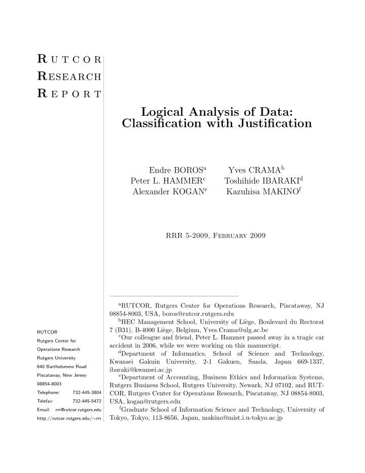
Page 20 RRR 5-2009 Figure 2: Results with the mushroom data set. Each point represents a pattern, the coor- dinates of which are the percentages of correctly classified training and test cases, when we use this pattern as a classifier. The horizontal scale is the percentage of correctly classified training cases, while the vertical axes represents the percentage of correctly classified test cases.

5 Empirical evidence

The focus of the present paper is primarily theoretical, as it aims at developing the notion of “justifiability”, and at analyzing the mathematical structure of the resulting concepts, pat- terns and bi-theories, in particular. Our line of arguing, however, naturally leads to favoring rules (in our case, patterns or co-patterns) which “fit well” the given data, as expressed by axiom (A2) in the Introduction of the paper. As is well known, such “maximalist” require- ment may possibly lead to overfitting, as many researchers observed in similar situations when using different classification approaches. For this reason, we feel important to stress that such overfitting behavior does not nec- essarily occur. This claim is based on extensive empirical evidence which has been reported elsewhere, and which we briefly summarize hereunder. First of all, there were several recent attempts in the literature to build patterns which have the highest coverage in the given training set and to use such patterns for classification, see e.g., [6, 7, 15, 18]. All of these papers reported good results, derived highly robust classifiers, and none experienced overfitting. We also designed various other computational experiments to test this behavior. In order to illustrate our point, we include here a small representative example. We considered some examples from the UC Irvine machine learning repository [3], chose randomly a small part

• f the data set as training set (typically 5-10%), left the rest as test data, and generated

RRR 5-2009 Page 21 exhaustively all patterns from the training set. For each pattern we computed the percentage

• f the training cases classified correctly by this pattern, as well as the percentage of the test

cases classified correctly. Thus each pattern is characterized by two percentages. We include here as illustration the results obtained for the so called “mushroom” data set. Figure 2 indicates the quality of the classification achieved by the 218 patterns which performed best

• n the training set; each of these patterns classified correctly at least 84% of the training

cases. What is even more surprising, however, is that the graph indicates a clear trend: Namely, those patterns performing better on the training set also perform better on the test set. Furthermore, even the variance of the test performance seems to decrease when the training performance increases. In fact we detected the same (sharp) tendency on all the data sets we tried. We view this as strong evidence supporting Dr P’s approach: Choosing the best performing patterns based on training set performance does not seem to lead to overfitting, and serves well our requirement to base classifications on the best available justification.

6 Future research

We can summarize our main contributions as follows: We introduced the notion of justifi- ability of a classifier, and concluded that all justifiable classifiers must be bi-theories. We also established that bi-theories are closely related to decision trees and nearest neighbor methods, but still form a larger class than those two produced by those classical methods. We also analyzed the structure of the pattern space in relation with bi-theories, and revealed the existence of various remarkable subsets of vectors (T −, T +, F −, F +) associated with an arbitrary pdBf (T, F). Many open questions emerge from our study: How much larger is the family of bi-theories than the family of decision trees? What is the proportion of bi-theories within the family

• f theories? Which Boolean functions can appear as maximal theories for a pdBf? How

difficult is to test whether T + = T (or F + = F)? How difficult is to generate T + and F +? We leave these questions for future research.

References

[1] H. Alhammady and K. Ramamohanarao, Using Emerging Patterns and Decision Trees in Rare-Class Classification, In: Proceedings of the Fourth IEEE International Confer- ence on Data Mining (ICDM’04), 315-318, 2004. [2] R. Agrawal, T. Imielinski and A. Swami, Mining association rules between sets of items in large databases, In: International Conference on Management of Data (SIGMOD 93), (1993), 207-216.

Page 22 RRR 5-2009 [3] A. Asuncion and D.J. Newman, UCI Machine Learning Repository [http://www.ics.uci.edu/ mlearn/MLRepository.html]. Irvine, CA: University

• f

California, School of Information and Computer Science. (2007) [4] L. Breiman, J.H. Friedman, R.A. Olshen and C.J. Stone, Classification and Regression Trees, Wadsworth International Group, 1984. [5] T.O. Bonates and P.L. Hammer, Large margin LAD classifiers. Technical Report RRR 22-2007, RUTCOR - Rutgers Center for Operations Research, Rutgers University, 2007. [6] T.O. Bonates and P.L. Hammer, A branch-and-bound algorithm for a family of pseudo- Boolean optimization problems. Technical Report RRR 21-2007, RUTCOR - Rutgers Center for Operations Research, Rutgers University, 2007. [7] T.O. Bonates, P.L. Hammer and A. Kogan, Maximum patterns in datasets, Discrete Applied Mathematics, 156(6) (2008) 846-861. [8] E. Boros, V. Gurvich, P.L. Hammer, T. Ibaraki and A. Kogan, Decomposability of partially defined Boolean functions, Discrete Applied Mathematics 62 (1995) pp. 51-75. [9] E. Boros, P.L. Hammer, T. Ibaraki, A. Kogan, E. Mayoraz and I. Muchnik, An im- plementation of logical analysis of data, IEEE Transactions on Knowledge and Data Engineering 12 (2000) 292-306. [10] E. Boros, P.L. Hammer, T. Ibaraki and A. Kogan, Logical analysis of numerical data, Mathematical Programming 79 (1997) pp. 163-190. [11] E. Boros, T. Ibaraki and K. Makino, Error-free and best-fit extensions of partially defined Boolean functions, Information and Computation 140 (2) (1998) pp. 254-283. [12] Y. Crama and P.L. Hammer, Boolean Functions – Theory, Algo- rithms, and Applications, Cambridge University Press, to appear (http://www.rogp.hec.ulg.ac.be/crama/). [13] Y. Crama, P.L. Hammer and T. Ibaraki, Cause-effect relationships and partially defined boolean functions, Annals of Operations Research 16 (1988) 299-326. [14] G. Dong and J. Li, Efficient mining of emerging patterns: discovering trends and dif- ferences, In: KDD ’99: Proceedings of the fifth ACM SIGKDD international conference

• n Knowledge discovery and data mining, (1999) 43-52.

[15] J. Eckstein, P.L. Hammer, Y. Liu, M. Nediak and B. Simeone, The maximum box prob- lem and its application to data analysis, Computational Optimization and Applications, 23(3):285298, 2002. [16] C. Flament, L’analyse bool´ eenne de questionnaires, Math´ ematiques et Sciences Hu- maines 12 (1966) 3-10.

RRR 5-2009 Page 23 [17] B. Ganter and R. Wille, Formal Concept Analysis - Mathematical Foundations, Springer-Verlag, Berlin, 1999. [18] N. Goldberg and Ch. Shan, Boosting optimal logical patterns, In: Proceedings of the Seventh SIAM International Conference on Data Mining Edited by Chid Apte, Bing Liu, Srinivasan Parthasarathy, and David Skillicorn, 2007. [19] P.L. Hammer, A. Kogan, B. Simeone and S. Szedmak. Pareto-optimal patterns in Log- ical Analysis of Data. Discrete Applied Mathematics, 144(1-2) (2004) pp. 79102. [20] L. Hyafil and R.L. Rivest, Constructing optimal binary decision trees is NP-complete, Information Processing Letters, 5 (1976) 15-17. [21] D. Kleitman, On Dedekind’s problem: The number of monotone Boolean functions, Proceedings of the American Mathematical Society 21 (1969) 677-682. [22] A. Kogan and Y. I. Zhuravlev, Realization of Boolean functions with a small number of zeros by disjunctive normal forms and related problems, Soviet Mathematics - Doklady (American Mathematical Society), 32 (3) (1985) 771-775. [23] A. Kogan, Disjunctive normal forms of Boolean functions with a small number of zeros, USSR Computational Mathematics and Mathematical Physics (Pergamon Press), 27 (3) (1987) 185-190. [24] A. Kogan, Lower bounds for the complexity of disjunctive normal forms of Boolean functions with a small number of zeros, USSR Computational Mathematics and Math- ematical Physics (Pergamon Press), 27 (6) (1987) 175-181. [25] K. Makino, T. Suda, T. Ono and T. Ibaraki, Data analysis by positive decision trees, IEICE Transactions on Information and Systems, Vol. E82-D, No.1, pp. 76-88, January 1999. [26] S. Muroga, Threshold Logic and its Applications, Wiley-Interscience, New York, 1971. [27] S.K. Murthy, S. Kasif and S. Salzberg, A system for induction of oblique decision trees, JAIR, 2 (1994) 1-32. [28] R. Potharst, J.C. Bioch and T. Petter, Monotone decision trees, Technical Report EUR- FEW-CS-97-07, Erasmus University, Rotterdam, 1997. [29] J.R. Quinlan, Induction of decision trees, Machine Learning 1 (1986) 81-106. [30] C.C. Ragin, The Comparative Method, University of California Press, Berkeley Los Angeles London, 1987.

Page 24 RRR 5-2009

A Proofs of main results

In this section we provide the proofs and necessary background of the results stated in Section 4.

A.1 Patterns and co-patterns

Let us first state an easy property of subcubes. Lemma A.1. If c ∈ [a, b] and c = b, then b ∈ [a, c].

• Proof. By definition of the subcube [a, b], c ∈ [a, b] means that cj = aj = bj for all indices

j ∈ {1, ..., n} for which aj = bj. Thus, c = b implies the existence of an index i such that ci = ai = bi, which then by the definition of subcubes implies that b ∈ [a, c]. Now we are ready to prove a main result about patterns and closures. Proof of Theorem 4.1. The second half of the claim follows from the first one by (ii) of Claim 3.4(ii). So, we concentrate on the first statement only. Let us denote by FT the family of all such subsets F ′ ⊆ Bn for which P(T, F ′) = P(T, F), and observe that by (iii) of Claim 3.4 we have F ′ ⊆ F ′′ ⊆ F ′′′ and F ′, F ′′′ ∈ FT imply F ′′ ∈ FT. Thus, to complete the proof of the theorem it is enough to show that FT has unique minimal and maximal elements. Let us next show that by (iii) of Claim 3.4 and by the definition of a pattern we have F ′, F ′′ ∈ FT implies F ′ ∪ F ′′ ∈ FT. (22) This is because if t is a pattern of both (T, F ′) and (T, F ′′), then we must have t(b) = 0 for all b ∈ F ′ ∪ F ′′, and t(a) = 1 for some a ∈ T. Thus, t is also a pattern of (T, F ′ ∪ F ′′), implying P(T, F ′) = P(T, F ′′) ⊆ P(T, F ′ ∪ F ′′), which together with (iii) of Claim 3.4 implies that P(T, F) = P(T, F ′ ∪ F ′′). Thus, (22) implies that FT has a unique maximal element, which we can denote by F +. To establish the existence of a unique minimal element F − in FT, it is enough to show that F ′, F ′′ ∈ FT implies F ′ ∩ F ′′ ∈ FT. (23) So, let us assume by contradiction that F ′, F ′′ ∈ FT but F ′∩F ′′ ∈ FT. Since (iii) of Claim 3.4 implies P(T, F ′) = P(T, F ′′) ⊆ P(T, F ′ ∩ F ′′), the assumption means that there is a term t ∈ P(T, F ′∩F ′′) which is not a member of P(T, F ′) = P(T, F ′′), or in other words, for which there exist vectors a ∈ T, b′ ∈ F ′ \ F ′′ and b′′ ∈ F ′′ \ F ′ such that t(a) = t(b′) = t(b′′) = 1. This means that T(t) is a subcube of Bn which intersects T, F ′ and F ′′, but does not intersect F ′∩F ′′. Let us then choose a minimal subcube included in T(t) and which intersects

RRR 5-2009 Page 25 both T and F ′ ∪ F ′′. Clearly, by Lemma A.1, such a minimal subcube contains exactly one vector from T and one vector from (F ′ ∪ F ′′) \ (F ′ ∩ F ′′). Let us assume, without any loss

• f generality that a ∈ T and b ∈ F ′ \ F ′′ are such vectors, and the minimal subcube is [a, b].

Then, the term t∗ defined by T(t∗) = [a, b] would be a pattern of (T, F ′′) but not a pattern of (T, F ′), contradicting our assumption that P(T, F ′) = P(T, F ′′). This contradiction proves

• ur claim, and hence completes the proof of the theorem.

Proof of Theorem 4.2 Assume that x ∈ Bn \ T is covered by some pattern t of (T, F). Then, by definition, t is not a pattern of (T, F ∪ {x}), and Theorem 4.1 implies that F ∪ {x} ⊆ F +, that is that x ∈ F +. Conversely, let x ∈ F +. Then, by Theorem 4.1, P(T, F) = P(T, F ∪ {x}). But this implies by (iii) of Claim 3.4 that there is a pattern of (T, F) which covers x. The statement about T + follows from the above by (ii) of Claim 3.4. It is easy to check that Corollary 4.3 immediately follows Theorem 4.2. Proof of Theorem 4.4 We want to prove that F + = F ∗, where F ∗ = {x ∈ Bn | [x, a] ∩ F = ∅ for all a ∈ T}. (24) To see that F + ⊆ F ∗, let us consider a vector x ∈ F ∗: thus, there exists a vector a ∈ T such that [x, a]∩F = ∅. For the term t defined by T(t) = [x, a], we have t(a) = 1 and t(b) = 0 for all b ∈ F; hence, t is a pattern of (T, F). Since this pattern covers x, Theorem 4.2 implies that x ∈ F +, and we conclude that F + ⊆ F ∗ as required. To see the equality, it is enough to show by (iii) of Claim 3.4 that P(T, F) ⊆ P(T, F ∗), since F ⊆ F ∗ by definition. Let us assume indirectly that t ∈ P(T, F)\P(T, F ∗), or in other words that t is a term for which t(b) = 0 for all b ∈ F, t(a) = 1 for some a ∈ T and t(x) = 1 for some x ∈ F ∗. Then we must have x ∈ F ∗ \ F, and [a, x] ⊆ T(t). However, by (24) we must have [a, x]∩F = ∅, proving that T(t)∩F = ∅, and hence contradicting the assumption that t is a pattern of (T, F). This contradiction proves the equality F + = F ∗, as claimed. To establish (11), let us denote by ˆ F the right hand side of this equality, i.e., ˆ F = {b ∈ F | ∃ a ∈ T such that [a, b] ∩ (F \ {b}) = ∅}. (25) We must prove that ˆ F = F − as defined in Theorem 4.1. We claim first that ˆ F ⊆ F −. Indeed, if b ∈ ˆ F \ F −, then there exists a ∈ T for which [a, b]∩(F \{b}) = ∅ by (25). The term t defined by T(t) = [a, b] is not a pattern of (T, F) since we have t(a) = t(b) = 1 for this particular a ∈ T and b ∈ F. Hence, by P(T, F) = P(T, F −), the term t cannot be a pattern of (T, F −), either. Since t(a) = 1 and a ∈ T, this implies that there exists a vector b′ ∈ F − for which t(b′) = 1, implying b′ ∈ [a, b]. Then, we have [a, b′] ⊆ [a, b], and by Lemma A.1 b ∈ [a, b′] is also implied. Let us then consider the term

Page 26 RRR 5-2009 t′ for which T(t′) = [a, b′]. Since [a, b′] ∩ F = ∅ by the above construction, t′ is a pattern

• f (T, F). However t′(b′) = 1 implies that t′ is not a pattern of (T, F −), contradicting the

definition of F −. Next, we claim that P(T, ˆ F) = P(T, F), which together with the previous claim and with the definition of F − will prove that ˆ F = F −. By (iii) of Claim 3.4, it in fact enough to show that P(T, ˆ F) ⊆ P(T, F). To verify this latter relation, let us assume indirectly that there exists a pattern t ∈ P(T, ˆ F) \ P(T, F). Consequently, we must have vectors a ∈ T and b ∈ F \ ˆ F such that t(a) = t(b) = 1. Since b ∈ ˆ F, we must have [a, b] ∩ (F \ {b}) = ∅ by (25). Since t is a pattern of (T, ˆ F) and, since T(t) ⊇ [a, b], all elements b′ ∈ [a, b] ∩ (F \ {b}) must belong to F \ ˆ F, and clearly [a, b′] ⊂ [a, b] holds for all such elements. Let us then choose a vector b′ ∈ [a, b] ∩ (F \ {b}) for which [a, b′] is a minimal sub-cube among all such sub-cubes. Since b′ ∈ ˆ F, there must exists another vector b′′ ∈ [a, b′] ∩ (F \ {b′}), and by the selection of b′ we must have b′′ ∈ ˆ

• F. However, t(b′′) = 1 follows from [a, b′] ⊆ T(t), contradicting the fact

that t was chosen as a pattern of (T, ˆ F). This contradiction proves that P(T, ˆ F) = P(T, F) as we claimed. The statements (12) and (13) follow from the above by interchanging the roles of T and F.

A.2 Maximal theories

Proof of Theorem 4.8 Let x ∈ Bn be an arbitrary binary vector and let a ∈ T ∪F be a vector closest to x in the sense of the Hamming distance. We can assume without any loss of generality that a ∈ T. Let us then consider the term t defined by T(t) = [x, a]. By Lemma A.1 we can assume that a ∈ T is the only vector from T ∪ F in [x, a], and hence t(b) = 0 must hold for all b ∈ F, implying that t is a pattern of (T, F). Hence, A(T,F)(x) = 1 must hold. Analogously, if a ∈ F, then we can derive that B(T,F)(x) = 1. This completes the proof of the first claim. The identities F(A(T,F)) = F + and F(B(T,F)) = T + are a mere restatement of Theo- rem 4.2, and the relation T + ∩ F + = ∅ follows readily from this fact and from the first claim. Proof of Theorem 4.10 Claim (i) follows readily by Theorem 4.8 and by the definition of patterns and co-patterns. To see (ii), let us consider an arbitrary pattern t of (T +, F +). By definition we have t(b) = 0 for all b ∈ F +, and thus T(t) ⊆ Bn \ F + = T(A(T,F)) follows from Theorem 4.8, implying that t is an implicant of A(T,F). Claim (iii) is implied by (i) and (ii). Proof of Theorem 4.11 To prove claim (iv), first note that any support set of (T +, F +) is also a support set of (T, F) since we have T + ⊇ T and F + ⊇ F. Therefore, let us consider a support set S of

RRR 5-2009 Page 27 (T, F) and show that it is also a support set of (T +, F +). If this were not true, there would exist two vectors a ∈ T + and b ∈ F + for which ai = bi for all i ∈ S. Assume without loss of generality that ai = bi = 1 for all i ∈ S and let t =

i∈S xi, so that we have

t(a) = 1 and t(b) = 1. (26) Now, let us choose a vector c ∈ T ∪F for which the cardinality of the set I = {i ∈ S : ci = 1} is as large as possible, and define the term t′ =

i∈I xi. Clearly, t′(c) = 1. Without any loss

• f generality, we can assume that c ∈ T (the case c ∈ F would be similar). Then, we claim

that t′(w) = 0 for all w ∈ F. Indeed, if t′(w) = 1 for some w ∈ F, then it means that wi = 1 for all i ∈ I. Since S is a support set of (T, F), there must be an index j ∈ S \ I such that wj = cj. Now, j ∈ I implies that cj = 0; hence this and wj = 1 contradicts the choice of c (since the set {i ∈ S : wi = 1} is larger than I). Thus, t′(w) = 0 for all w ∈ F, and t′(c) = 1, meaning that t′ is a pattern of (T, F). Then t′(b) = 0 follows from Theorem 4.2 and from the assumption that b ∈ F +. Since t ≤ t′, we conclude that t(b) = 0, which contradicts the second equality in (26).

A.3 Decision trees and bi-theories

Recall the definition of reasonable decision trees given at the end of Section 3.2. Such decision trees offer an algorithmic representation of Boolean functions and of pdBfs. They are widely used in machine learning, data mining, and other fields. Moreover, as we shall see, they feature a close relationship with bi-theories. Example A.2. Figure 3 shows an example of a decision tree D. This decision tree classifies, for instance, all binary vectors for which x1 = x2 = x5 = 1 into the rightmost leaf belonging to L1. Thus, we have fD(1, 1, x3, x4, 1) = 1 for all x3, x4. For each node v ∈ N∪L of a decision tree D, let us denote by Pv = {r = u0, u1, ..., uk = v} the unique path from the root r to v. We can associate an elementary conjunction tv with v by defining tv =

• ui∈Pv:

ui+1 is the right successor of ui

xj(ui)

• ∧
• ui∈Pv:

ui+1 is the left successor of ui

xj(ui)

• .

In words, we include the literal xj in tv if the path Pv follows the right successor from a node u ∈ Pv with j(u) = j, and we include xj if Pv follows the left successor. It is then immediate to see that DNF representations of fD and f D are given by fD =

• v∈L1(D)

tv and f D =

• v∈L0(D)

tv. (27)

Page 28 RRR 5-2009

✒✑ ✓✏ ✒✑ ✓✏ ✒✑ ✓✏ ✒✑ ✓✏

1 1

• ❅

❅ ❅ ❅ ❅ ❅ ❅ ❅ ❅ ❅

• ❅

❅ ❅ ❅ ❅

r label = 2 v1 label = 1 v2 label = 5

x2 = 0 x2 = 1 x1 = 0 x1 = 1 x5 = 0 x5 = 1 Figure 3: An example of a decision tree. Example A.3. The decision tree D in Figure 3 has two leaves in L1(D), and thus we obtain the following DNF for the function represented by D: fD = x1x2 ∨ x1x2x5. Considering the leaves in L0(D) we get f D = x2 ∨ x1x2x5. It is well-known that every pdBf (T, F) with T ∩F = ∅ can be represented by a reasonable decision tree. Here, we provide a generic procedure to build such a decision tree D ∈ D(T, F), and we establish some properties of our procedure in Theorem A.4. With every node v of D (to be built), let us associate the pdBf (Tv, Fv), consisting of those vectors of T and F, respectively, which are classified into node v. During the execution

• f the proposed algorithm we maintain a list Q of nodes v such that

Tv ∪ Fv = ∅ and Tv ∩ Fv = ∅. (28)

RRR 5-2009 Page 29 DT-Build(T, F) Initialize: Let N = Q = {r}, L1 = L0 = ∅, A(D) = ∅, Tr = T and Fr = F. (Upon completion, the vertex set N ∪ L0 ∪ L1 and the arc set A(D) define the constructed decision tree.) While Q = ∅ do Choose a node u ∈ Q and remove it from Q. If Tu = ∅, then add u to L0. If Fu = ∅, then add u to L1. If Tu = ∅ and Fu = ∅, then choose an index j such that xj is not constant for all x ∈ Tu ∪ Fu, and set j(u) = j. Let v and w, respectively, be the left and right successors of u, and define the associated pdBfs by Tv = {a ∈ Tu | aj = 0} and Fv = {b ∈ Fu | bj = 0}, Tw = {a ∈ Tu | aj = 1} and Fw = {b ∈ Fu | bj = 1}. Finally, add both v and w to Q and N, and add the arcs (u, v) and (u, w) to the set of arcs A(D). Theorem A.4. For every pdBf (T, F), the algorithm DT-Build(T, F) produces a reasonable decision tree D ∈ D(T, F). Moreover, all reasonable decision trees in D(T, F) arise in this way.

• Proof. Let us note first that Tv ∪ Fv = ∅ and Tw ∪ Fw = ∅ holds in the above algorithm

for the successors v and w of a node u if and only if the index j = j(u) is chosen so that xj is not a constant in all vectors x ∈ Tv ∪ Fv. Furthermore, if Tu ∩ Fu = ∅, then we have both Tv ∩ Fv = ∅ and Tw ∩ Fw = ∅. Thus, conditions (28) are indeed maintained during the procedure, assuming that we had initially T ∩ F = ∅. Let us also remark that as long as Tu = ∅, Fu = ∅, and Tu ∩ Fu = ∅, there must exist an index j for which xj is not constant in all x ∈ Tu ∪ Fu. After the data splitting at each vertex u, we have xj(u) = 1 in all vectors x ∈ Tz ∪ Fz for all nodes z belonging to the subtree rooted at the right successor w of u. Similarly, we have xj(u) = 0 for all vectors x ∈ Tz ∪ Fz for all nodes z belonging to the subtree rooted at the left successor v of u. This implies that the same index will not be selected twice along any of the paths going from the root to a leaf. Let us finally observe that every time we add a node u to either L0 or L1, the corre- sponding pdBf (Tu, Fu) contains some vectors, due to condition (28). Therefore, the decision tree D produced by DT-Build(T, F) indeed represents (T, F) and it is reasonable. We can also see that the total number of leaves is not more than |T ∪F|,

Page 30 RRR 5-2009 and hence the procedure terminates in O(|T ∪ F|) steps. It is obvious that every decision tree D for (T, F) can be produced by DT-Build, since it suffices to choose the indices j(u) as prescribed by D. Corollary A.5. If (T, F) is a pdBf, then D(T, F) = ∅. Many variants of DT-Build are proposed in the literature, differing (only) in the way

• f choosing the splitting index j = j(u) in each iteration. One of the best-known procedures

is the algorithm ID3 due to Quinlan [29]. A.3.1 Properties of decision trees as bi-theories Let us now analyze the connection between decision trees and patterns, co-patterns, theories, and co-theories. Lemma A.6. For a decision tree D ∈ D(T, F) and for a leaf node v of D, the corresponding term tv is a pattern of (T, F) if v ∈ L1(D), while it is a co-pattern of (T, F) if v ∈ L0(D).

• Proof. This is almost immediate by the definitions. For instance, if v ∈ L1(D), then Tv = ∅

and Fv = ∅, implying that tv(a) = 1 for all a ∈ Tv and tv(b) = 0 for all b ∈ F. Proof of Theorem 4.13 Let us consider an arbitrary reasonable decision tree of (T, F). By Corollary A.5 there are such decision trees. Then by Lemma A.6 every term of fD (and f D), given by (27) is a pattern (co-pattern). Consequently fD is a bi-theory. Before we turn to a proof of Theorem 4.15, we need an additional defintion. Let us call a term t a prime pattern (prime co-pattern) of a pdBf (T, F) if it is a pattern (co- pattern) of (T, F) but every term obtained by dropping anyone of its literals is not a pattern (co-pattern). In other words, when viewed as either Boolean functions or subcubes, prime patterns (prime co-patterns) are maximal patterns (co-patterns). Lemma A.7. Every prime pattern t of (T, F) appears as t = tv for some decision tree D ∈ D(T, F) and for some true leaf v ∈ L1(D). Similarly, every prime co-pattern t of (T, F) appears as t = tu for some decision tree D ∈ D(T, F) and for some false leaf u ∈ L0(D).

• Proof. Let us prove the statement for prime patterns. The case of prime co-patterns can be

treated analogously. Let t =

ji∈P(t) xji

• ji∈N(t) xji be a prime pattern of (T, F), let P(t) ∪ N(t) = {ji | i =

1, ..., k}, and let us consider a small decision tree D∗ consisting of one path u1, u2, ..., uk+1. Here u1 is the root of D∗, and ui+1 is the right successor of ui if ji ∈ P(t), and it is the left successor if ji ∈ N(t). Let vi denote the other successor of vertex ui, i = 1, ..., k, and set L1(D∗) = {uk+1} and L0(D∗) = {v1, v2, ..., vk}.

RRR 5-2009 Page 31 Let us now note that Fuk+1 = {b ∈ F | t(b) = 1} = ∅ and Tuk+1 = {a ∈ T | t(a) = 1} = ∅ since t is a pattern of (T, F). Since t is prime, it does not remain a pattern if any variable xji is deleted from it. Thus there must exist a vector b ∈ F for which bji = aji for some i and bjℓ = ajℓ for ℓ = i, where a ∈ T is an arbitrary vector for which t(a) = 1. Therefore, Fvi = {b ∈ F | bji = aji and bjℓ = ajℓ, ℓ < i} = ∅. Since this is true for all indices ji, i = 1, ..., k, every node of D∗ has some vectors of T ∪ F classified into it. Then let us choose an arbitrary decision tree Di ∈ D(Tvi, Fvi) and identify the root of Di with vi, for i = 1, ..., k. In this way we obtain a decision tree D for which we have D ∈ D(T, F) and in which t appears as t = tuk+1. This lemma allows us to give one more characterization of the closure (T +, F +) of a pdBf (T, F). Proof of Theorem 4.15 Let us first show the equivalence (a) ⇐ ⇒ (b). Note that no decision tree D ∈ D(T, F) can classify a vector v ∈ T + into a false leaf, or a vector u ∈ F + into a true leaf, since every decision tree D ∈ D(T, F) represents a bi-theory of (T, F) by Theorem 4.13, and since T + = F(B(T,F)) and F + = F(A(T,F)) by Theorem 4.8. Thus, to complete the proof of this equivalence we only need to show that no vectors u ∈ T + or u ∈ F + have the same property. For this, let us consider a vector u ∈ T +. Then, by the definition (12), there exists a vector b ∈ F such that [u, b]∩T = ∅. Thus the term t defined by T(t) = [u, b] is a co-pattern

• f (T, F). Let t′ ≥ t be a prime co-pattern of (T, F). Then, by Lemma A.7 there exists a

decision tree D ∈ D(T, F) for which t′ = tv for some leaf v ∈ L0(D). This decision tree classifies u into the false leaf v, showing that not all decision trees in D(T, F) classify u into a true leaf, as claimed. The case of a vector u ∈ F + is similarly handled. To see the equivalence (a) ⇐ ⇒ (c), let us note that (c) = ⇒ (b) = ⇒ (a) by Theorem 4.13 and the above proof. Furthermore, Corollary 4.3 implies (a) = ⇒ (c), thus completing

• ur proof.

A.4 Nearest neighbor methods and bi-theories

The following useful property can be deduced from (18)–(19): It states that if u lies between a and v, then v is closer to u than to a. Lemma A.8. For all vectors a, u, v ∈ Bn, if u ∈ [a, v] and a = u, then ρ(u, v) < ρ(a, v) when ρ is a subcube monotone similarity measure.

• Proof. Let u ∈ [a, v]. Condition (19) implies that, if we indirectly assume ρ(a, v) ≤ ρ(u, v),

then ρ(a, u) ≤ ρ(u, u) = 0. Hence ρ(a, u) = 0, and (18) implies that a = u, a contradiction. Proof of Theorem 4.16

Page 32 RRR 5-2009 Let us note first that since T ∩ F = ∅, we have for all a ∈ T and b ∈ F: ρ(a, F) > 0 = ρ(a, a) = ρ(a, T) and ρ(b, T) > 0 = ρ(b, b) = ρ(b, F), by (18) and (20). Thus T ⊆ T(fρ) and F ⊆ F(fρ), implying that fρ ∈ E(T, F). To see that fρ is a theory, let us associate with every vector v ∈ T(fρ) the term t[v,a] defined by T(t[v,a]) = [v, a], where a ∈ T is any vector such that ρ(v, a) = ρ(v, T), and let us define ϕ =

• v∈T(fρ)

t[v,a]. We want to show that ϕ is a theory and that ϕ = fρ. Let us first show that every term t[v,a], v ∈ T(fρ), is a pattern of (T, F). Clearly, the term t[v,a] covers a point of T (namely, a). Moreover, suppose that t[v,a] covers a point of F, say u ∈ F ∩[v, a]. Then, by Lemma A.8, ρ(u, v) < ρ(a, v), which contradicts the assumption that v ∈ T(fρ). Thus, for all v ∈ T(fρ), t[v,a] intersects T and does not intersect F, meaning that t[v,a] is a pattern of (T, F), and that ϕ is a theory. We claim next that this theory is fρ, that is, T(ϕ) = T(fρ). (29) Clearly, for all v ∈ T(fρ), the term t[v,a] covers v, and hence ϕ(v) = 1; this shows that T(fρ) ⊆ T(ϕ). For the converse inclusion, consider an arbitrary vector u ∈ T(ϕ), and let t[v,a], v ∈ T(fρ), be any term of ϕ which covers u: u ∈ T(t[v,a]) = [v, a]. For every vector b ∈ F, we have by definition of fρ that ρ(v, T) = ρ(a, v) ≤ ρ(b, v); hence, (19) implies ρ(a, u) ≤ ρ(b, u). Since this holds for all b ∈ F, we conclude that ρ(u, T) ≤ ρ(u, F), hence fρ(u) = 1. This establishes the claim (29). Finally, to see that fρ is a bi-theory, we have to show that its complement f ρ is a co- theory of (T, F). To this end, let us associate with every vector w ∈ F(fρ) the term t[w,b] defined by T(t[w,b]) = [w, b], where b ∈ F is a vector for which ρ(w, b) = ρ(w, F), and define ψ =

• w∈F(fρ)

t[w,b]. By similar arguments as above, it follows that all terms of ψ are co-patterns, and that T(ψ) = F(fρ). Thus, f ρ is a co-theory of (T, F), which completes the proof of the theorem. As mentioned earlier, many mappings ρ : Bn × Bn → R+ are subcube monotone simi- larity measures. The Hamming distance provides a simple example. We describe below a large family of subcube monotone mappings which generalize the Hamming distance (the Hamming distance is obtained when ωj = 1 for all j = 1, 2, . . . , n). Lemma A.9. Let ωj > 0 be positive real numbers for j = 1, 2, . . . , n, and let ρω(a, b) =

• j:aj=bj

ωj for all a, b ∈ Bn. (30) Then ρω is a subcube monotone similarity measure.

RRR 5-2009 Page 33

• Proof. Condition (17) holds trivially, and condition (18) follows from the positivity of ωj for

j = 1, 2, . . . , n. To see condition (19), let us consider arbitrary binary vectors a, b, u and v, such that u ∈ [v, a], and let us define the following index sets A = {j | aj = vj = uj = bj}, B = {j | aj = vj = uj = bj}, C = {j | aj = bj = uj = vj}, D = {j | bj = uj = vj = aj}, E = {j | aj = bj = uj = vj}, F = {j | aj = uj = bj = vj}. These sets are pairwise disjoint, and since u ∈ [v, a], we have V = A ∪ B ∪ C ∪ D ∪ E ∪ F. To simplify notation, we write ω(S) instead of

j∈S ωj. Then we have

ρω(a, v)=ω(C ∪ D ∪ E ∪ F) ρω(b, v)=ω(B ∪ C ∪ E) ρω(a, u)=ω(D ∪ E), ρω(b, u)=ω(B ∪ E ∪ F). By elementary computations, ρω(b, v) − ρω(a, v) = ω(B ∪ C ∪ E) − ω(C ∪ D ∪ E ∪ F) = ω(B) − ω(D ∪ F) ≤ ω(B) − ω(D ∪ F) + 2ω(F) = ω(B ∪ F) − ω(D) = ω(B ∪ E ∪ F) − ω(D ∪ E) = ρω(b, u) − ρω(a, u) using the facts that the sets B, C, D, E and F are pairwise disjoint, and that ω(F) ≥ 0 by the nonnegativity of ω. Condition (19) then follows immediately.