
R Modules for Accurate and Reliable Statistical Computing
Micah Altman (Harvard University) Jeff Gill (University of California, Davis) Michael P. McDonald (George Mason University; Brookings Institution)
Micah Altman, Harvard University R Modules for Accurate and Reliable Statistica 2
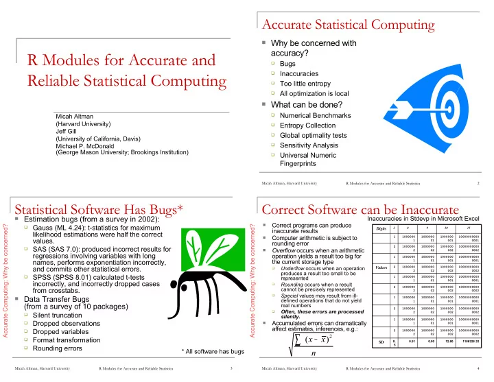
Accurate Statistical Computing
Why be concerned with
accuracy?
Bugs Inaccuracies Too little entropy All optimization is local
What can be done?
Numerical Benchmarks Entropy Collection Global optimality tests Sensitivity Analysis Universal Numeric
Fingerprints
Micah Altman, Harvard University R Modules for Accurate and Reliable Statistica 3
Statistical Software Has Bugs*
Estimation bugs (from a survey in 2002):
Gauss (ML 4.24): t-statistics for maximum
likelihood estimations were half the correct values.
SAS (SAS 7.0): produced incorrect results for
regressions involving variables with long names, performs exponentiation incorrectly, and commits other statistical errors.
SPSS (SPSS 8.01) calculated t-tests
incorrectly, and incorrectly dropped cases from crosstabs.
Data Transfer Bugs
(from a survey of 10 packages)
Silent truncation Dropped observations Dropped variables Format transformation Rounding errors
Accurate Computing: Why be concerned? * All software has bugs
Micah Altman, Harvard University R Modules for Accurate and Reliable Statistica 4
Correct Software can be Inaccurate
Correct programs can produce inaccurate results
Computer arithmetic is subject to rounding error
Overflow occurs when an arithmetic
- peration yields a result too big for
the current storage type
Underflow occurs when an operation produces a result too small to be represented
Rounding occurs when a result cannot be precisely represented
Special values may result from ill- defined operations that do not yield real numbers
Often, these errors are processed silently.
Accumulated errors can dramatically affect estimates, inferences, e.g.:
n x x
∑
−
2
) (
:
Inaccuracies in Stdevp in Microsoft Excel Accurate Computing: Why be concerned?
SD Values Digits
0. 5 2 1 2 1 2 1 2 1 2 1 2 0.51 1000000 2 1000000 1 1000000 2 1000000 1 1000000 2 1000000 1 1000000 2 1000000 1 1000000 2 1000000 1 8 0.00 1000000 02 1000000 01 1000000 02 1000000 01 1000000 02 1000000 01 1000000 02 1000000 01 1000000 02 1000000 01 9 12.80 1000000 002 1000000 001 1000000 002 1000000 001 1000000 002 1000000 001 1000000 002 1000000 001 1000000 002 1000000 001 10 1186328.32 10000000000 0002 10000000000 0001 10000000000 0002 10000000000 0001 10000000000 0002 10000000000 0001 10000000000 0002 10000000000 0001 10000000000 0002 10000000000 0001 15