SLIDE 1 Quiz
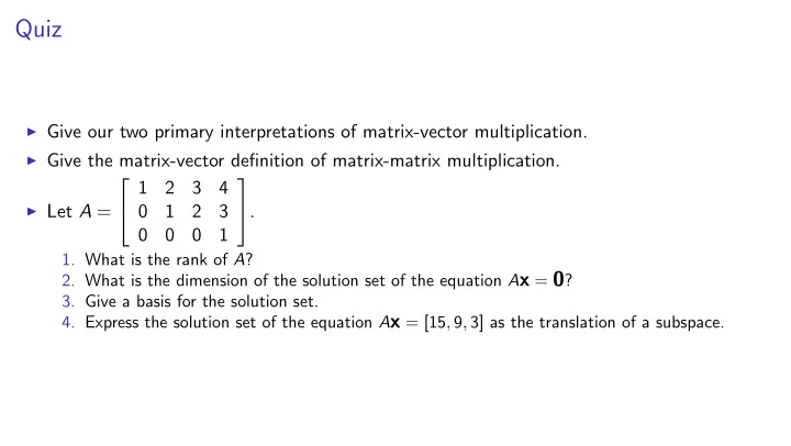
I Give our two primary interpretations of matrix-vector multiplication. I Give the matrix-vector definition of matrix-matrix multiplication. I Let A =
2 4 1 2 3 4 1 2 3 1 3 5.
- 1. What is the rank of A?
- 2. What is the dimension of the solution set of the equation Ax = 0?
- 3. Give a basis for the solution set.
- 4. Express the solution set of the equation Ax = [15, 9, 3] as the translation of a subspace.
SLIDE 2
Vector-matrix multiplication
We interpret m-vector as m × 1 matrix (“column vector”) v = 2 4 1 2 3 3 5 Can transpose to get 1 × m matrix (“row vector”) vT = ⇥ 1 2 3 ⇤ . We know two ways to interpret matrix-vector multiplication:
I Linear-combinations interpretation: Av is linear combination of columns of A I Dot-product interpretation: Entry r of Av is dot-product of row r of A with v.
What about multiplying a row vector by a matrix? ⇥ 1 2 3 ⇤ 2 4 1 5 1 10 1 4 3 5 Use transpose rule ((AB)T = BTAT): @⇥ 1 2 3 ⇤ 2 4 1 5 1 10 1 4 3 5 1 A
T
= 2 4 1 5 1 10 1 4 3 5
T
⇥ 1 2 3 ⇤T = 1 1 1 5 10 4 2 4 1 2 3 3 5 Now can use familiar interpretations of matrix-vector product Can we obtain interpretations of original vector-matrix product?
SLIDE 3
Vector-matrix multiplication
We interpret m-vector as m × 1 matrix (“column vector”) v = 2 4 1 2 3 3 5 Can transpose to get 1 × m matrix (“row vector”) vT = ⇥ 1 2 3 ⇤ . We know two ways to interpret matrix-vector multiplication:
I Linear-combinations interpretation: Av is linear combination of columns of A I Dot-product interpretation: Entry r of Av is dot-product of row r of A with v.
What about multiplying a row vector by a matrix? ⇥ 1 2 3 ⇤ 2 4 1 5 1 10 1 4 3 5 Use transpose rule ((AB)T = BTAT): @⇥ 1 2 3 ⇤ 2 4 1 5 1 10 1 4 3 5 1 A
T
= 2 4 1 5 1 10 1 4 3 5
T
⇥ 1 2 3 ⇤T = 1 1 1 5 10 4 2 4 1 2 3 3 5 Now can use familiar interpretations of matrix-vector product Can we obtain interpretations of original vector-matrix product?
SLIDE 4
Vector-matrix multiplication
We interpret m-vector as m × 1 matrix (“column vector”) v = 2 4 1 2 3 3 5 Can transpose to get 1 × m matrix (“row vector”) vT = ⇥ 1 2 3 ⇤ . We know two ways to interpret matrix-vector multiplication:
I Linear-combinations interpretation: Av is linear combination of columns of A I Dot-product interpretation: Entry r of Av is dot-product of row r of A with v.
What about multiplying a row vector by a matrix? ⇥ 1 2 3 ⇤ 2 4 1 5 1 10 1 4 3 5 Use transpose rule ((AB)T = BTAT): @⇥ 1 2 3 ⇤ 2 4 1 5 1 10 1 4 3 5 1 A
T
= 2 4 1 5 1 10 1 4 3 5
T
⇥ 1 2 3 ⇤T = 1 1 1 5 10 4 2 4 1 2 3 3 5 Now can use familiar interpretations of matrix-vector product Can we obtain interpretations of original vector-matrix product?
SLIDE 5 Quiz
For each item in the left column, list every letter corresponding to an item in the right column that always fits. By fits, I don’t mean that something is always true. I mean that it makes sense—that it “type-checks”.
- 1. Dimension of ...
- 2. Rank of ...
- 3. Span of ...
- 4. Col space of ...
- 5. Row space of ...
- 6. Null space of ...
- 7. kernel of ...
- 8. ... is one-to-one
- 9. ... is onto
- 10. ... is invertible
- 11. ... is trivial
(a) vector space/subspace (b) affine space (c) vector (d) matrix (e) linear combination (f) linear transformation (g) set of vectors
SLIDE 6
Quiz, continued: Uniqueness of representation.
Let b1, . . . , bn be a basis for a vector space V. Use the definition of basis to show that each vector in V has exactly one (at least one and at most one) representation in terms of b1, . . . , bn.
SLIDE 7
Echelon form
Definition: An m × n matrix A is in echelon form if it satisfies the following condition: for any row, if that row’s first nonzero entry is in position k then every previous row’s first nonzero entry is in some position less than k. This definition implies that, as you iterate through the rows of A, the first nonzero entries per row move strictly right, forming a sort of staircase that descends to the right. 2 6 6 4 2 3 5 6 1 3 4 1 2 9 3 7 7 5
1 3 1 2 2 6 3 4 1 1 7 9 3 1 4 1 2
2 6 6 4 4 1 3 3 1 1 7 9 3 7 7 5
SLIDE 8
Sorting rows by position of the leftmost nonzero
Goal: a method of transforming a rowlist into one that is in echelon form. First attempt: Sort the rows by position of the leftmost nonzero entry. We will use a naive algorithm of sorting:
I first choose a row with a nonzero in first column, I then choose a row with a nonzero in second column,
. . . accumulating these in a list new rowlist, initially empty: new_rowlist = [] The algorithm maintains the set of indices of rows remaining to be sorted, rows left, initially consisting of all the row indices: rows_left = set(range(len(rowlist)))
SLIDE 9 Sorting rows by position of the leftmost nonzero
col_label_list = sorted(rowlist[0].D, key=str) new_rowlist = [] rows_left = set(range(len(rowlist)))
I Algorithm iterates through the column labels in order. I In each iteration, algorithm finds a list
rows with nonzero
- f indices of the remaining rows that have nonzero entries in the current column
I Algorithm selects one of these rows (the pivot row), adds it to new rowlist,
and removes its index from rows left. for c in col_label_list: rows_with_nonzero = [r for r in rows_left if rowlist[r][c] != 0] pivot = rows_with_nonzero[0] new_rowlist.append(rowlist[pivot]) rows_left.remove(pivot)
SLIDE 10
Sorting rows by position of the leftmost nonzero
for c in col label list: rows with nonzero = [r for r in rows left if rowlist[r][c] != 0] if rows with nonzero != []: pivot = rows with nonzero[0] new rowlist.append(rowlist[pivot]) rows left.remove(pivot) Run the algorithm on 2 6 6 4 2 3 4 5 5 1 2 3 4 5 4 5 3 7 7 5 new rowlist
I After first two iterations, new rowlist is [[1, 2, 3, 4, 5], [0, 2, 3, 4, 5]], and rows left is
{1, 3}.
I The algorithm runs into trouble in third iteration since none of the remaining rows have a
nonzero in column 2.
I In this case, the algorithm should just move on to the next column without changing
new rowlist or rows left.
SLIDE 11
Sorting rows by position of the leftmost nonzero
for c in col label list: rows with nonzero = [r for r in rows left if rowlist[r][c] != 0] if rows with nonzero != []: pivot = rows with nonzero[0] new rowlist.append(rowlist[pivot]) rows left.remove(pivot) Run the algorithm on 2 6 6 4 2 3 4 5 5 1 2 3 4 5 4 5 3 7 7 5 new rowlist ⇥ 1 2 3 4 5 ⇤
I After first two iterations, new rowlist is [[1, 2, 3, 4, 5], [0, 2, 3, 4, 5]], and rows left is
{1, 3}.
I The algorithm runs into trouble in third iteration since none of the remaining rows have a
nonzero in column 2.
I In this case, the algorithm should just move on to the next column without changing
new rowlist or rows left.
SLIDE 12 Sorting rows by position of the leftmost nonzero
for c in col label list: rows with nonzero = [r for r in rows left if rowlist[r][c] != 0] if rows with nonzero != []: pivot = rows with nonzero[0] new rowlist.append(rowlist[pivot]) rows left.remove(pivot) Run the algorithm on 2 6 6 4 2 3 4 5 5 1 2 3 4 5 4 5 3 7 7 5 new rowlist 1 2 3 4 5 2 3 4 5
- I After first two iterations, new rowlist is [[1, 2, 3, 4, 5], [0, 2, 3, 4, 5]], and rows left is
{1, 3}.
I The algorithm runs into trouble in third iteration since none of the remaining rows have a
nonzero in column 2.
I In this case, the algorithm should just move on to the next column without changing
new rowlist or rows left.
SLIDE 13
Sorting rows by position of the leftmost nonzero
for c in col label list: rows with nonzero = [r for r in rows left if rowlist[r][c] != 0] if rows with nonzero != []: pivot = rows with nonzero[0] new rowlist.append(rowlist[pivot]) rows left.remove(pivot) Run the algorithm on 2 6 6 4 2 3 4 5 5 1 2 3 4 5 4 5 3 7 7 5 new rowlist 2 4 1 2 3 4 5 2 3 4 5 4 5 3 5
I After first two iterations, new rowlist is [[1, 2, 3, 4, 5], [0, 2, 3, 4, 5]], and rows left is
{1, 3}.
I The algorithm runs into trouble in third iteration since none of the remaining rows have a
nonzero in column 2.
I In this case, the algorithm should just move on to the next column without changing
new rowlist or rows left.
SLIDE 14
Sorting rows by position of the leftmost nonzero
for c in col label list: rows with nonzero = [r for r in rows left if rowlist[r][c] != 0] if rows with nonzero != []: pivot = rows with nonzero[0] new rowlist.append(rowlist[pivot]) rows left.remove(pivot) Run the algorithm on 2 6 6 4 2 3 4 5 5 1 2 3 4 5 4 5 3 7 7 5 new rowlist 2 6 6 4 1 2 3 4 5 2 3 4 5 4 5 5 3 7 7 5
I After first two iterations, new rowlist is [[1, 2, 3, 4, 5], [0, 2, 3, 4, 5]], and rows left is
{1, 3}.
I The algorithm runs into trouble in third iteration since none of the remaining rows have a
nonzero in column 2.
I In this case, the algorithm should just move on to the next column without changing
new rowlist or rows left.
SLIDE 15
Flaw in sorting
for c in col label list: rows with nonzero = [r for r in rows left if rowlist[r][c] != 0] if rows with nonzero != []: pivot = rows with nonzero[0] new rowlist.append(rowlist[pivot]) rows left.remove(pivot) rowlist new rowlist 2 6 6 4 2 3 4 5 3 2 1 2 3 4 5 6 7 3 7 7 5 ⇒ 2 6 6 4 1 2 3 4 5 2 3 4 5 3 2 6 7 3 7 7 5 Result is not in echelon form. Need to introduce another transformation....
SLIDE 16
Elementary row-addition operations
2 6 6 4 2 3 4 5 3 2 1 2 3 4 5 6 7 3 7 7 5 ⇒ 2 6 6 4 2 3 4 5 3 2 1 2 3 4 5 3 3 7 7 5 Repair the problem by changing the rows: Subtract twice the second row 2 [0, 0, 0, 3, 2] from the fourth [0, 0, 0, 6, 7] gettting new fourth row [0, 0, 0, 6, 7] − 2 [0, 0, 0, 3, 2] = [0, 0, 0, 6 − 6, 7 − 4] = [0, 0, 0, 0, 3] The 3 in the second row is called the pivot element. That element is used to zero out another element in same column.
SLIDE 17
Elementary row-addition operations
Transformation is multiplication by a elementary row-addition matrix: 2 6 6 4 1 1 1 −2 1 3 7 7 5 2 6 6 4 2 3 4 5 3 2 1 2 3 4 5 6 7 3 7 7 5 = 2 6 6 4 2 3 4 5 3 2 1 2 3 4 5 3 3 7 7 5 Such a matrix is invertible: 2 6 6 4 1 1 1 −2 1 3 7 7 5 and 2 6 6 4 1 1 1 2 1 3 7 7 5 are inverses. We will show: Proposition: If MA = B where M is invertible then Row A = Row B. Therefore change to row causes no change in row space. Therefore basis for changed rowlist is also a basis for original rowlist.
SLIDE 18
Preserving row space
Lemma: Row NA ⊆ Row A. Proof: Let v be any vector in Row NA. That is, v is a linear combination of the rows of NA. By the linear-combinations definition of vector-matrix multiplication, there is a vector u such that
v =
⇥
uT
⇤ @ 2 4 N 3 5 2 4 A 3 5 1 A = @⇥
uT
⇤ 2 4 N 3 5 1 A 2 4 A 3 5 by associativity which shows that v can be written as a linear combination of the rows of A. QED
SLIDE 19
Preserving row space
Lemma: Row NA ⊆ Row A. Proposition: If M is invertible then Row MA = Row A Proof: Must show Row MA ⊆ Row A and Row A ⊆ Row MA
I Lemma shows Row MA ⊆ Row A. I Let B = MA I M has an inverse M−1
⇒ M−1B = A
I Lemma shows Row M−1B
| {z }
A
⊆ Row B |{z}
MA I That is, Row A ⊆ Row MA
QED
SLIDE 20
Gaussian elimination
Applying elementary row-addition operations does not change the row space. Incorporate into the algorithm for c in col label list: rows with nonzero = [r for r in rows left if rowlist[r][c] != 0] if rows with nonzero != []: pivot = rows with nonzero[0] rows left.remove(pivot) new rowlist.append(rowlist[pivot]) add suitable multiple of rowlist[pivot] to each row in rows with nonzero[1:] 2 6 6 4 1 2 3 4 2 3 4 5 3 4 5 6 4 5 6 7 3 7 7 5 ⇒ 2 6 6 4 1 2 3 4 −1 −2 −3 −2 −4 −6 −3 −6 −9 3 7 7 5 ⇒ 2 6 6 4 1 2 3 4 −1 −2 −3 3 7 7 5 To avoid problems due to round-off error, let’s work over GF(2)
SLIDE 21
Gaussian elimination
Applying elementary row-addition operations does not change the row space. Incorporate into the algorithm for c in col label list: rows with nonzero = [r for r in rows left if rowlist[r][c] != 0] if rows with nonzero != []: pivot = rows with nonzero[0] rows left.remove(pivot) new rowlist.append(rowlist[pivot]) for r in rows with nonzero[1:]: multiplier = rowlist[r][c]/rowlist[pivot][c] rowlist[r] -= multiplier * rowlist[pivot] 2 6 6 4 1 2 3 4 2 3 4 5 3 4 5 6 4 5 6 7 3 7 7 5 ⇒ 2 6 6 4 1 2 3 4 −1 −2 −3 −2 −4 −6 −3 −6 −9 3 7 7 5 ⇒ 2 6 6 4 1 2 3 4 −1 −2 −3 3 7 7 5 To avoid problems due to round-off error, let’s work over GF(2)
SLIDE 22 Gaussian elimination for GF(2)
A B C D 1 1 X 1 1 1 1 2 1 1 3 1 1 1 1 A: Select row 1 as pivot. Put it in new rowlist Since rows 2 and 3 have nonzeroes, we must add row 1 to rows 2 and 3. new rowlist ⇥ 1 1 1 ⇤ A B C D 1 1 X 1 1 1 1 2 1 X 3 1 B: Select row 3 as pivot. Put it in new rowlist Other remaining rows have zeroes in column B, so no row additions needed. new rowlist 1 1 1 1
B C D X 1 1 X 1 1 1 1 2 1 X 3 1 C: Select row 0 as pivot . Put it in new rowlist. Only other remaining row is row 2, and we add row 0 to row 2. new rowlist 2 4 1 1 1 1 1 1 3 5
SLIDE 23
Gaussian elimination for GF(2)
new rowlist 2 4 1 1 1 1 1 1 3 5 A B C D X 1 1 X 1 1 1 1 X 2 1 X 3 1 D: Only remaining row is row 2, so select it as pivot row. Put it in new rowlist No other rows, so no row additions. new rowlist 2 6 6 4 1 1 1 1 1 1 1 3 7 7 5 We are done.