Quiz! How costly is this operation (naive solution)? course per - - PDF document

1

Database Systems

Indexes

DBMSs and ”NoSQL”

1

Quiz!

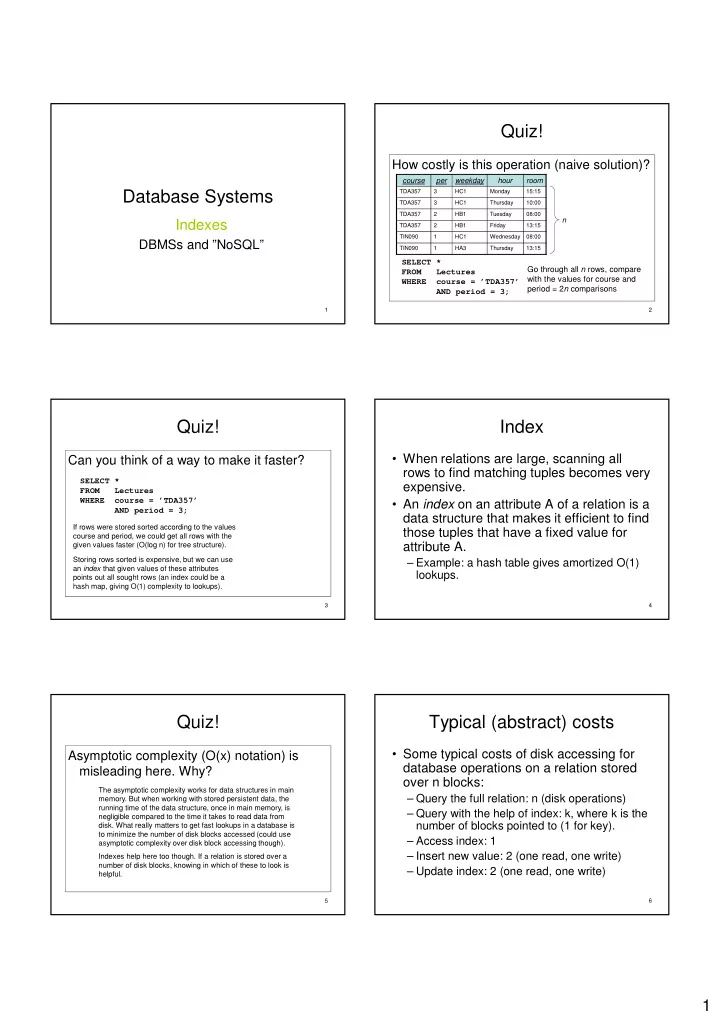
How costly is this operation (naive solution)?

SELECT * FROM Lectures WHERE course = ’TDA357’ AND period = 3;

course per weekday hour room

TDA357 3 HC1 Monday 15:15 TDA357 3 HC1 Thursday 10:00 TDA357 2 HB1 Tuesday 08:00 TDA357 2 HB1 Friday 13:15 TIN090 1 HC1 Wednesday 08:00 TIN090 1 HA3 Thursday 13:15

n

Go through all n rows, compare with the values for course and period = 2n comparisons

2

Quiz!

Can you think of a way to make it faster?

SELECT * FROM Lectures WHERE course = ’TDA357’ AND period = 3;

If rows were stored sorted according to the values course and period, we could get all rows with the given values faster (O(log n) for tree structure). Storing rows sorted is expensive, but we can use an index that given values of these attributes points out all sought rows (an index could be a hash map, giving O(1) complexity to lookups).

3

Index

• When relations are large, scanning all

rows to find matching tuples becomes very expensive.

• An index on an attribute A of a relation is a

data structure that makes it efficient to find those tuples that have a fixed value for attribute A.

– Example: a hash table gives amortized O(1) lookups.

4

Quiz!

Asymptotic complexity (O(x) notation) is misleading here. Why?

The asymptotic complexity works for data structures in main

• memory. But when working with stored persistent data, the

running time of the data structure, once in main memory, is negligible compared to the time it takes to read data from

• disk. What really matters to get fast lookups in a database is

to minimize the number of disk blocks accessed (could use asymptotic complexity over disk block accessing though). Indexes help here too though. If a relation is stored over a number of disk blocks, knowing in which of these to look is helpful.

5

Typical (abstract) costs

• Some typical costs of disk accessing for

database operations on a relation stored

• ver n blocks:

– Query the full relation: n (disk operations) – Query with the help of index: k, where k is the number of blocks pointed to (1 for key). – Access index: 1 – Insert new value: 2 (one read, one write) – Update index: 2 (one read, one write)

6

2

Example:

SELECT * FROM Lectures WHERE course = ’TDA357’ AND period = 3;

Assume Lectures is stored in n disk blocks. With no index to help the lookup, we must look at all rows, which means looking in all n disk blocks for a total cost of n. With an index, we find that there are 2 rows with the correct values for the course and period attributes. These are stored in two different blocks, so the total cost is 3 (2 blocks + reading index).

7

Quiz!

How costly is this operation?

SELECT * FROM Lectures, Courses WHERE course = code;

Go through all n blocks in Lectures, compare the value for course from each row with the values for code in all rows of Courses, stored in all m

• blocks. The total cost is thus n * m

accessed disk blocks.

Lectures: n disk blocks Courses: m disk blocks

Index on code in Courses: No index: Go through all n blocks in Lectures, compare the value for course from each row with the index. Since course is a key, each value will exist at most once, so the cost is 2 * n + 1 accessed disk blocks (1 for fetching the index once).

8

CREATE INDEX

• Most DBMS support the statement

CREATE INDEX index name ON table (attributes); – Example: – Statement not in the SQL standard, but most DBMS support it anyway. – Primary keys are given indexes implicitly (by the SQL standard).

CREATE INDEX courseIndex ON Courses (code);

9

Important properties

• Indexes are separate data stored by itself.

Can be created

• n newly created relations
• n existing relations
• will take a long time on large relations.

Can be dropped without deleting any table data.

• SQL statements do not have to be

changed

– a DBMS automatically uses any indexes.

10

Quiz!

Why don’t we have indexes on all attributes for faster lookups?

– Indexes require disk space. – Modifications of tables are more expensive.

• Need to update both table and index.

– Not always useful

• The table is very small.
• We don’t perform lookups over it (Note: lookups queries).

– Using an index costs extra disk block accesses.

11

Rule of thumb

• Mostly queries on tables – use indexes for

key attributes.

• Mostly updates – be careful with indexes!

12

3

Quiz!

Assume we have an index on Lectures for (course, period, weekday) which is the key. How costly are these queries?

SELECT * FROM Lectures WHERE course = ’TDA357’ AND period = 3; Lectures: n disk blocks SELECT * FROM Lectures WHERE weekday = ’Monday’ AND room = ’HC1’;

A multi-attribute index is typically organized hierarchically. First the rows are indexed according to the first attribute, then according to the second within each group, and so on. Thus the left query costs at most k + 1 where k is the number of rows matching the values. The right query can’t use the index, and thus costs n, where n is the size of the relation in disk blocks.

13

Example: Suppose that the Lectures relation is stored in 20 disk blocks, and that we typically perform three operations on this table:

– insert new lectures (Ins) – list all lectures of a particular course (Q1) – list all lectures in a given room (Q2)

Let’s assume that in an average week there are:

– 2 lectures for each course, and – 10 lectures in each room.

Let’s also assume that

– each course has lectures stored in 2 blocks, and – each room has lectures stored in 7 (some lectures are stored in the same block).

14

Example continued:

The amortized cost depends on the distribution of the operations. p1 is proportion of operations that are Q1 queries, p2 similarly for Q2, and thus the proportion of operations that are Ins modifications is 1 – p1 – p2. For some different values of p1 and p2 we get actual costs of:

6 – 3p1 + 2p2 4 + 16p1 + 4p2 4 – p1 + 16p2 2 + 18p1 + 18p2 cost 8 8 20 20 Q2 3 20 3 20 Q1 6 4 4 2 Ins Both indexes Index for room Index for (course, period, weekday) No index Indexes 2 + 18p1 + 18p2 4 – p1 + 16p2 4 + 16p1 + 4p2 6 – 3p1 + 2p2 p1 = p2 = 0.4 16.4 10 12 5.6 p1 = p2 = 0.1 5.6 5.5 6 5.9 p1 = 0.6, p2 = 0.3 18.2 8.2 14.8 4.8

Insert new lectures (Ins) List all lectures of a particular course (Q1) List all lectures in a given room (Q2)

15

Quiz!

• Indexes are incredibly useful (although they are

not part of the SQL standard).

• Doing it wrong is costly.
• Requires knowledge about the internals of a

DBMS.

– How is data stored? How large is a block?

• A DBMS should be able to decide better than

the user what indexes are needed, from usage analysis. So why don’t they??

16

Summary – indexes

• Indexes make certain lookups and joins more

efficient.

– Disk block access matters. – Multi-attribute indexes

• CREATE INDEX
• Usage analysis

– What are the expected operations? – How much do they cost? (cost of operation)x(fraction of time on operation)

17

RDBMSs and beyond

The NoSQL movement

18

4

(R)DBMSs ”today”

DMBS

• Approx. market share

Oracle 40% IBM DB2 30% Microsoft SQL Server 15% Sybase 3%

(…)

MySQL 1% PostgreSQL 0.5% (Microsoft Access)

19

Proprietary RDBMSs

• Oracle DB

– First commercial SQL database – HUGE market share historically – Standard incompliant

• IBM DB2

– First SQL database (in-house) – Near-monopoly on ”mainframes” – Towards Oracle-compliant (!)

• Microsoft SQL Server

– Market leading on Windows application platforms

20

MySQL

• Open Source – but owned by Oracle since 2010
• Historically: fast but feature-poor

– Subqueries (!) added in recent release – FK constraints only with non-standard backend – ACID transactions only (crudely) with non-standard backends – Not optimized for joins

• Still missing features (but getting closer)

– No CHECK constraints (including assertions) – No sequencing (WITH)

• Big on the web: used by Wikipedia, Facebook, …

– Early support in PHP helped boost

21

PostgreSQL

• Open Source – community development
• Historically: full-featured but (relatively) slow
• Much faster today – and optimized for complex tasks

– Efficient support for joins

• Almost standard-compliant

– Full constraint support – except assertions! – Full ACID transactions – Sequencing (WITH)

• Prominent users: Yahoo, MySpace, Skype, …

22

Beyond SQL?

• SQL was first developed around 1970

– Contemporaries: Forth, PL/I, Pascal, C, SmallTalk, ML, …

• With one prominent exception – C – these have

all been succeded by newer, cooler languages.

• Has the time finally come for SQL as well?

23

SQL injection attacks

http://xkcd.com/327/ The possibility for SQL injection attacks has lead development away from literal SQL, towards higher-level interfaces, tools and libraries.

24

5

The world is a-changin’

• ”The Claremont Report”, 2008

– Big Data is coming big-time

• Social networks, e-science, Web 2.0, streaming media, …

– Data IS the business

• Efficient data management is no longer just a cost reduction

– it’s a selling point!

– Rapidly expanding user base

• … means rapidly expanding user needs

– Architectural shifts in computing

• Storage hardware is still improving exponentially
• Data networks, cloud computing, …

25

Examples of database sizes

• Digg: 3 TB – just to store the up/down

votes

• Facebook: 50 TB – for the private

messaging feature

• eBay: 2 PB data overall (2 000 000 GB)

26

RDBMS weakness

• RDBMSs typically handle ”massive” amounts of

data in complex domains, with frequent small read/writes.

– The archetypical RDBMS serves a bank.

• Data-intensive applications don’t fit this pattern:

– MASSIVE+++ amounts of data (e.g. eBay) – Super-fast indexing of documents (e.g. Google) – Serving pages on high-traffic websites (e.g. Facebook) – Streaming media (e.g. Spotify)

27

Column-oriented databases

• Typical RDBMSs are row-oriented

– All data associated with a particular key is stored close together. – Allows horizontal partitioning (sharding)

• Different rows stored on different distributed nodes.
• Column-oriented (R)DBMSs

– All data in a given column is stored close together. – Allows vertical partitioning (normalization)

• Different columns stored on different nodes.

– Fast computation of aggregations, e.g. data mining.

28

The ”NoSQL” movement

• NoSQL (”Not only SQL”)

– Originally the name of an RDBMS with a different interface language. – Nowadays a term that encompasses a wide variety of non-relational DBMSs (”NoRel”?).

SELECT fun, profit FROM Real_World WHERE relational = FALSE;

29

Non-relational databases

• MapReduce framework

– Google originally; Hadoop (Apache), …

• Key-Value stores

– BigTable (Google), Cassandra (Apache), …

• Document stores

– CouchDB, MongoDB, SimpleDB, …

• Graph databases

– Neo4j, …

• Semi-structured databases

– (Native) XML databases

30

6

MapReduce

• No data model – all data stored in files
• Operations supplied by user:

– Reader :: file → [input record] – Map :: input record → <key, value> – Reduce :: <key, [value]> → [output record] – Writer :: [output record] → file

• Everything else done behind the scenes:

– Consistency, atomicity, distribution and parallelism, ”glue”

• Optimized for broad data analytics

– Running simple queries over all data at once

31

MapReduce implementations

• The ”secret” behind Google’s success

– Still going strong.

• Hadoop (Apache)

– Open Source implementation of the MapReduce framework – Used by Ebay, Amazon, Last.fm, LinkedIn, Twitter, Yahoo, Facebook internal logs (~15PB), …

32

Key-Value Stores

• Key-Value stores is a fancy name for

persistant maps (associative arrays):

• Extremely simple interface – extremely

complex implementations.

void Put(string key, byte[] data); byte[] Get(string key); void Remove(string key);

33

Key-Value Stores

• Built for extreme efficiency, scalability and fault

tolerance

– Records distributed to different nodes based on key – Replication of data to several nodes

• Sacrifice consistency and querying power

– Single-record transactions – Not good for ”joins” – ”Eventual consistency” between nodes

• AKA: ”why does Facebook tell me I have a notification when

there isn’t anything new when I click the icon??!?”

34

Key-Value store implementations

• BigTable (Google)

– Sparse, distributed, multi-dimensional sorted map – Proprietary – used in Google’s internals: Google Reader, Google Maps, YouTube, Blogger, …

• Cassandra (Apache)

– Originally Facebook’s PM database – now Open Source (Apache top-level project) – Used by Netflix, Digg, Reddit, Spotify, …

35

Document stores

• Roughly: Key-Value stores where the

values are ”documents”

– XML, JSON, mixed semistructured data sets

• Typically incorporate a query language for

the document type.

– See next lecture for discussion on XML querying.

36

7

Graph Databases

• Data modeled in a graph structure

– Nodes = ”entities” – Properties = ”tags”, attribute values – Edges connect

• Nodes to nodes (relationships)
• Nodes to properties (attributes)
• Fast access to associative data sets

– All entities that share a common property – Computing association paths

• Used by Twitter (FlockDB) to store user relations, …

37

Semi-structured data (SSD)

• More flexible than the relational model.

– The type of each ”entity” is its own business. – Labels indicate meanings of substructures.

• Semi-structured: it is structured, but not everything is

structured the same way!

• Special case: Document databases (see above)
• The data model behind XML – more on this next lecture!

38

NoSQL – a hype?

• NoSQL is not ”the right choice” just because it’s new!
• Relational DBMSs still rule at what they were first

designed for: efficient access to large amounts of data in complex domains. That’s still the vast majority!

39

NoSQL summary

• NoSQL = ”Not only SQL”
• Different data models optimized for

different tasks

– MapReduce, Key-Value stores, Document stores, Graph databases, …

• Typically:

+ efficiency, scalability, flexibility, fault tolerance

• (no) query language, (less) consistency

40

Next lecture

Semi-structured data XML

41