Quickselect algorithm Divide-Conquer-Glue Algorithms Quicksort, - - PowerPoint PPT Presentation

Divide-Conquer-Glue Algorithms

Quicksort, Quickselect and the Master Theorem Tyler Moore

CS 2123, The University of Tulsa

Some slides created by or adapted from Dr. Kevin Wayne. For more information see http://www.cs.princeton.edu/~wayne/kleinberg-tardos. Some code reused from Python Algorithms by Magnus Lie Hetland.

Quickselect algorithm

Selection Problem: find the kth smallest number of an unsorted sequence. What is the name for selection when k = n

2?

Θ(n lg n) solution is easy. How? There is a linear-time solution available in the average case

2 / 20

Partitioning with pivots

To use a divide-conquer-glue strategy, we need a way to split the problem in half Furthermore, to make the running time linear, we need to always identify the half of the problem where the kth element is Key insight: split the sequence by a random pivot. If the subset of smaller items happens to be of size k − 1, then you have found the

• pivot. Otherwise, pivot on the half known to have k.

3 / 20

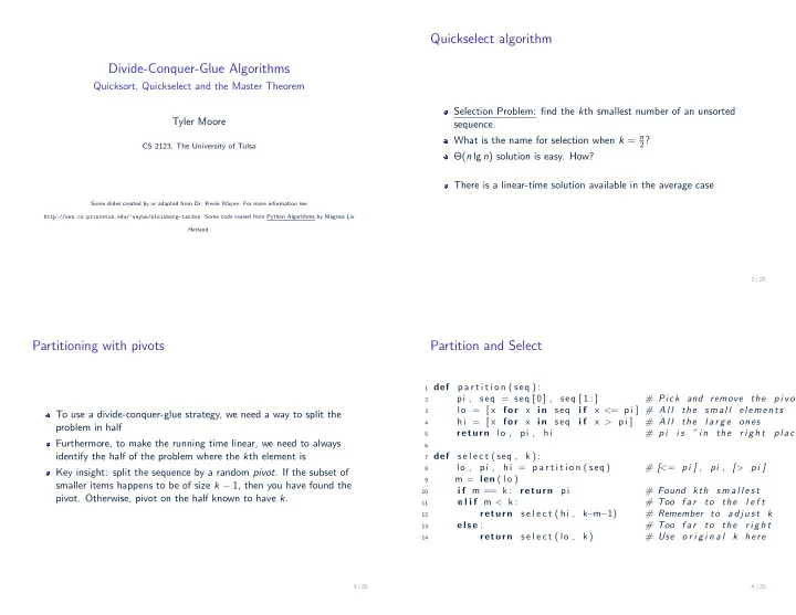
Partition and Select

1 def

p a r t i t i o n ( seq ) :

2

pi , seq = seq [ 0 ] , seq [ 1 : ] # Pick and remove the p i v o t

3

l o = [ x for x in seq i f x <= pi ] # A l l the small elements

4

hi = [ x for x in seq i f x > pi ] # A l l the l a r g e

• nes

5

return lo , pi , hi # pi i s ” in the r i g h t place

6 7 def

s e l e c t ( seq , k ) :

8

lo , pi , hi = p a r t i t i o n ( seq ) # [<= pi ] , pi , [> pi ]

9

m = len ( l o )

10

i f m == k : return pi # Found kth s m a l l e s t

11

e l i f m < k : # Too f a r to the l e f t

12

return s e l e c t ( hi , k− m−1) # Remember to a d j u s t k

13

else : # Too f a r to the r i g h t

14

return s e l e c t ( lo , k ) # Use

• r i g i n a l

k here

4 / 20

A verbose Select function

def s e l e c t ( seq , k ) : lo , pi , h i = p a r t i t i o n ( seq ) # [<= p i ] , pi , [> p i ] p r i n t lo , pi , h i m = len ( l o ) p r i n t ’ s m a l l p a r t i t i o n l e n g t h %i ’ %(m) i f m == k : p r i n t ’ found kth s m a l l e s t %s ’ % p i return p i # Found kth s m a l l e s t e l i f m < k : # Too f a r to the l e f t p r i n t ’ s m a l l p a r t i t i o n has %i elements , so kth must be i n r i g h t sequence ’ % m return s e l e c t ( hi , k− m−1) # Remember to a d j u s t k e l s e : # Too f a r to the r i g h t p r i n t ’ s m a l l p a r t i t i o n has %i elements , so kth must be i n l e f t sequence ’ % m return s e l e c t ( lo , k ) # Use

• r i g i n a l

k here

5 / 20

Seeing the Select in action

>>> select([3, 4, 1, 6, 3, 7, 9, 13, 93, 0, 100, 1, 2, 2, 3, 3, 2],4) [1, 3, 0, 1, 2, 2, 3, 3, 2] 3 [4, 6, 7, 9, 13, 93, 100] small partition length 9 small partition has 9 elements, so kth must be in left sequence [0, 1] 1 [3, 2, 2, 3, 3, 2] small partition length 2 small partition has 2 elements, so kth must be in right sequence [2, 2, 3, 3, 2] 3 [] small partition length 5 small partition has 5 elements, so kth must be in left sequence [2, 2] 2 [3, 3] small partition length 2 small partition has 2 elements, so kth must be in left sequence [2] 2 [] small partition length 1 found kth smallest 2 2

6 / 20

From Quickselect to Quicksort

Question: what if we wanted to know all k-smallest items (for k = 1 → n)?

1 def

q u i c k s o r t ( seq ) :

2

i f len ( seq ) <= 1: return seq # Base case

3

lo , pi , hi = p a r t i t i o n ( seq ) # pi i s in i t s place

4

return q u i c k s o r t ( l o ) + [ pi ] + q u i c k s o r t ( hi ) # Sort l o and hi s e p a r a t e l y

7 / 20

Best case for Quicksort

The total partitioning on each level is O(n), and it take lg n levels of perfect partitions to get to single element subproblems. When we are down to single elements, the problems are sorted. Thus the total time in the best case is O(n lg n).

8 / 20

Worst case for Quicksort

Suppose instead our pivot element splits the array as unequally as possible. Thus instead of n/2 elements in the smaller half, we get zero, meaning that the pivot element is the biggest or smallest element in the array. Now we have n1 levels, instead of lg n, for a worst case time of Θ(n2), since the first n/2 levels each have ≥ n/2 elements to partition.

9 / 20

Picking Better Pivots

Having the worst case occur when they are sorted or almost sorted is very bad, since that is likely to be the case in certain applications. To eliminate this problem, pick a better pivot:

1

Use the middle element of the subarray as pivot.

2

Use a random element of the array as the pivot.

3

Perhaps best of all, take the median of three elements (first, last, middle) as the pivot. Why should we use median instead of the mean?

Whichever of these three rules we use, the worst case remains O(n2).

10 / 20

Randomized Quicksort

Suppose you are writing a sorting program, to run on data given to you by your worst enemy. Quicksort is good on average, but bad on certain worst-case instances. If you used Quicksort, what kind of data would your enemy give you to run it on? Exactly the worst-case instance, to make you look bad. But instead of picking the median of three or the first element as pivot, suppose you picked the pivot element at random. Now your enemy cannot design a worst-case instance to give to you, because no matter which data they give you, you would have the same probability of picking a good pivot!

11 / 20

Randomized Guarantees

Randomization is a very important and useful idea. By either picking a random pivot or scrambling the permutation before sorting it, we can say: “With high probability, randomized quicksort runs in Θ(n lg n) time” Where before, all we could say is: “If you give me random input data, quicksort runs in expected Θ(n lg n) time.” See the difference?

12 / 20

Importance of Randomization

Since the time bound how does not depend upon your input distribution, this means that unless we are extremely unlucky (as

• pposed to ill prepared or unpopular) we will certainly get good

performance. Randomization is a general tool to improve algorithms with bad worst-case but good average-case complexity. The worst-case is still there, but we almost certainly wont see it.

13 / 20

Recurrence Relations

Recurrence relations specify the cost of executing recursive functions. Consider mergesort

1

Linear-time cost to divide the lists

2

Two recursive calls are made, each given half the original input

3

Linear-time cost to merge the resulting lists together

Recurrence: T(n) = 2T( n

2) + Θ(n)

Great, but how does this help us estimate the running time?

14 / 20

Master Theorem Extracts Time Complexity from Some Recurrences

Definition

The Master Theorem For any recurrence relation of the form T(n) = aT(n/b) + c · nk , T(1) = c, the following relationships hold: T(n) =      Θ(nlogb a) if a > bk Θ(nk log n) if a = bk Θ(nk) if a < bk. So what’s the complexity of Mergesort? Mergesort recurrence: T(n) = 2T( n

2) + Θ(n)

Since a = 2, b = 2, k = 1, 2 = 21. Thus T(n) = Θ(nk log n)

15 / 20

Apply the Master Theorem

Definition

The Master Theorem For any recurrence relation of the form T(n) = aT(n/b) + c · nk , T(1) = c, the following relationships hold: T(n) =      Θ(nlogb a) if a > bk Θ(nk log n) if a = bk Θ(nk) if a < bk. Let’s try another one: T(n) = 3T( n

5) + 8n2

Well a = 3, b = 5, c = 8, k = 2, and 3 < 52. Thus T(n) = Θ(n2)

16 / 20

Apply the Master Theorem

Definition

The Master Theorem For any recurrence relation of the form T(n) = aT(n/b) + c · nk , T(1) = c, the following relationships hold: T(n) =      Θ(nlogb a) if a > bk Θ(nk log n) if a = bk Θ(nk) if a < bk. Now it’s your turn: T(n) = 4T( n

2) + 5n

17 / 20

What’s going on in the three cases?

Definition

The Master Theorem For any recurrence relation of the form T(n) = aT(n/b) + c · nk , T(1) = c, the following relationships hold: T(n) =      Θ(nlogb a) if a > bk Θ(nk log n) if a = bk Θ(nk) if a < bk.

1 Too many leaves: leaf nodes outweighs sum of divide and glue costs 2 Equal work per level: split between leaves matches divide and glue

costs

3 Too expensive a root: divide and glue costs dominate 18 / 20

Quicksort Recurrence (Average Case)

1 def

q u i c k s o r t ( seq ) :

2

i f len ( seq ) <= 1: return seq # Base case

3

lo , pi , hi = p a r t i t i o n ( seq ) # pi i s in i t s place

4

return q u i c k s o r t ( l o ) + [ pi ] + q u i c k s o r t ( hi ) # Sort l o and hi s e p a r a t e l y T(n) = 2T( n

2) + Θ(n), so T(n) = n log n

19 / 20

Selection (Average Case)

1 def

s e l e c t ( seq , k ) :

2

lo , pi , hi = p a r t i t i o n ( seq ) # [<= pi ] , pi , [> pi ]

3

m = len ( l o )

4

i f m == k : return pi # Found kth s m a l l e s t

5

e l i f m < k : # Too f a r to the l e f t

6

return s e l e c t ( hi , k− m−1) # Remember to a d j u s t k

7

else : # Too f a r to the r i g h t

8

return s e l e c t ( lo , k ) # Use

• r i g i n a l

k here

20 / 20