
SLIDE 1
Elliptic Curve Cryptography
Jim Royer
CIS 428/628: Introduction to Cryptography
November 6, 2018
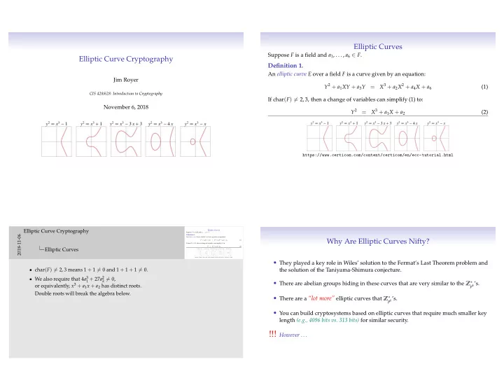
Elliptic Curves
Suppose F is a field and a1, . . . , a6 ∈ F.
Definition 1.
An elliptic curve E over a field F is a curve given by an equation: Y2 + a1XY + a3Y = X3 + a2X2 + a4X + a6 (1) If char(F) = 2, 3, then a change of variables can simplify (1) to: Y2 = X3 + a1X + a2 (2)
https://www.certicom.com/content/certicom/en/ecc-tutorial.html
Elliptic Curves
Suppose F is a field and a1, . . . , a6 ∈ F. Definition 1. An elliptic curve E over a field F is a curve given by an equation: Y2 + a1XY + a3Y = X3 + a2X2 + a4X + a6 (1) If char(F) = 2, 3, then a change of variables can simplify (1) to: Y2 = X3 + a1X + a2 (2) https://www.certicom.com/content/certicom/en/ecc-tutorial.html
2018-11-06
Elliptic Curve Cryptography Elliptic Curves
- char(F) = 2, 3 means 1 + 1 = 0 and 1 + 1 + 1 = 0.
- We also require that 4a3
1 + 27a2 2 = 0,
- r equivalently, x3 + a1x + a2 has distinct roots.
Double roots will break the algebra below.
Why Are Elliptic Curves Nifty?
- They played a key role in Wiles’ solution to the Fermat’s Last Theorem problem and
the solution of the Taniyama-Shimura conjecture.
- There are abelian groups hiding in these curves that are very similar to the Z∗
pk’s.
- There are a “lot more” elliptic curves that Z∗
pk’s.
- You can build cryptosystems based on elliptic curves that require much smaller key